Introduction

Writing algorithms is a good way of learning the "ways", or better, the expressiveness of the rust language.

Merge Algorithms

Merging two or more ordered sets

The basic use case for these algorithms is merging two ordered arrays into a single and ordered array. Although simple, it becomes far more complicated when you consider

• Very large datasets spanning many processing nodes (segmentation, map/reduce, etc)
• Memory and cpu constraints on embedded systems (in-place, out-of-place)

Benchmarks

The following benchmarks provide an indicative performance comparison between the different merge implementations. The input size used is 5,000 (2 x 2,500) elements.

Out of place merge function
===========================
test bench_merge_iterator          ... bench:      61,250 ns/iter (+/- 5,708)

In place merge functions
========================
test bench_merge_lazy              ... bench:      80,606 ns/iter (+/- 2,367)
test bench_merge_mut               ... bench:      68,282 ns/iter (+/- 8,597)
test bench_merge_mut_adjacent      ... bench:      43,533 ns/iter (+/- 655)

Implementation

The chapters that follow, provide a detailed explanation on how the below implementation works

/// Applies memory efficient in-place merging when two slices are adjacent to each other.
/// ```
/// use csx3::merge::merge_mut_fast;
///
/// let mut input = vec![1, 3, 5, 7, 9, 2, 4, 6, 8, 10];
/// let (s1,s2) = input.split_at_mut(5);
///
/// merge_mut_fast(s1,s2);
/// assert_eq!(input, vec![1,2,3,4,5,6,7,8,9,10]);
/// ```
/// Panics in case the two slices are found not to be adjacent. For safety, always use *ONLY* against slices that have been mutable split from an existing slice
pub fn merge_mut_fast<T>(s1: &mut [T], s2: &mut [T]) -> usize where T: Ord + Debug {
    let ws: &mut [T];

    unsafe {
        ws = from_raw_parts_mut(s1.as_mut_ptr(), s1.len() + s2.len());
        assert!(s2[0] == ws[s1.len()]);
    }

    let (mut p, mut c, mut j, llen, mut inversion ) = (0usize, 0usize, s1.len(), s1.len(), 0usize);
    let mut idx_rfl: Vec<usize> = Vec::from_iter(0..ws.len());
    let len = idx_rfl.len();

    //println!("{ws:?}::{idx_rfl:?}, ({i},{c},{j})");

    unsafe {
        let idxp = idx_rfl.as_mut_ptr();
        let wsp = ws.as_mut_ptr();

        let mut cc; // c' definition
        let mut pp; // p' definition

        loop {
            cc = *idxp.add(c);
            pp = *idxp.add(p);
            match (j < len && j != p, p < len-1 && c < llen -1) {
                (true, _) if (*wsp.add(cc)).cmp(&(*wsp.add(j))) == Ordering::Greater => {
                    inversion += j - p;
                    wsp.add(p).swap( wsp.add(j));
                    //idx_rfl.swap(ii, j);
                    idxp.add(pp).write(j);
                    idxp.add(j).write(pp);
                    j += 1;
                },
                (_, true) => {
                    wsp.add(p).swap(wsp.add(cc));
                    //idx_rfl.swap(pp, c);
                    idxp.add(cc).write(pp);
                    idxp.add(pp).write(cc);
                    c += 1;
                },
                (_,_) => break,
            };
            p += 1;
            //println!("{ws:?}::{idx_rfl:?}, ({i},{c},{j})");
        }
    }
    //println!("Merge Done!");
    inversion
}

In-place Merge Algorithm with O(n+m) swaps

General Approach

In an "In place" merge of two ordered arrays it is always required to maintain a pivot between merged and unmerged sub-arrays as we go over the process of

1. Use comparison indexes (c,j) to find the smallest element between (a) the left and (b) right ordered arrays
2. Swap the next smallest element of the left and right sub-arrays against a pivot position (p)
3. Repeat until we've exhausted comparing and swapping of all elements

Start                               Finish
==============================     ==========================
Left array       Right array       Ordered elements across arrays
+---+---+---+    +---+---+---+     +---+---+---+  +---+---+---+
| 1 | 3 | 5 | <> | 2 | 4 | 6 | =>  | 1 | 2 | 3 |  | 4 | 5 | 6 |
+---+---+---+    +---+---+---+     +---+---+---+  +---+---+---+
  c                j

Generic Approach of using a pivot to separate 
"merged" from "yet to be merged" regions
=============================================

         | left        Right  |
         | [c]         [j]    |
+---+---+|+---+---+   +---+---+ 
| 1 | 2 ||| 3 | 5 |   | 4 | 6 | 
+---+---+|+---+---+   +---+---+ 
Merged   |     Unmerged region  
region   p: Pivot

Challenge

Taking a naive first step

By trying to swap the smallest element of the two arrays with the pivot we quickly realise that things are getting out of control very soon. For example,

                              c  j  p   [c] > [j]  Action
 c/p             j            =======   =========  ========================
[(1 , 3 , 5)]  [(2 , 4 , 6)]  1  1  1    1     2   left swap(c,p) incr(c,p)
     c/p         j                  
[ 1 ,(3 , 5)]  [(2 , 4 , 6)]  2  1  2    3     2   right swap(j,p) incr(j,p)
      c   p          j                   
[ 1 , 2 ,(5 ]  [ 3),(4 , 6)]  2  2  3    2!!   4   Fail: We lost control here! 2 isn't part of the left array

At this stage our partitioned region is left of p and equal to [1,2] while the unmerged region is [(5!!,3),(4,6)] which is clearly out-of-order and the result from then on is unpredictable. During the 2nd iteration, the left comparison index [c] points to a 2 rather 3 which is now at the 4th position in the right array, or the 2nd position in the unmerged partition. Therefore, we need to find a way to maintain a solid comparison index reference [c] for the left array while we iterate through

Problem Solution

Canceling the Rotation during right swaps

It becomes obvious that during the right swap operation our left array is rotated left as seen below

                              c  j  p   [c] > [j]  Action
 c/p             j            =======   =========  ========================
[(1 , 3 , 5)]  [(2 , 4 , 6)]  1  1  1    1     2   left swap(c,p) incr(c,p)
     c/p         j                   
[ 1 ,(3 , 5)]  [(2 , 4 , 6)]  2  1  2    3     2   right swap(j,p) incr(j,p)
      c   p          j                  
[ 1 , 2 ,(5 ]  [ 3),(4 , 6)]  <-- Here instead of [3,5] we have [5,3]

Moreover, the partition point [p] more or less points to the where the left comparison index [c] should have been, that is, the unmerged partition. Let's try this time with

• reverting the rotation effect after each right swap hence bringing the left unmerged part back to order
• using [c] as both the partition and the left comparison index

                              c  j    [c] > [j]  Action
  c              j            ====    =========  ============================
[(1 , 3 , 5)]  [(2 , 4 , 6)]  1  1     1     2   No swap, just incr(c)
      c          j                   
[ 1 ,(3 , 5)]  [(2 , 4 , 6)]  2  1     3     2   right swap(j,c), incr(c,j)
          c          j 
[ 1 , 2 ,(5 ]  [ 3),(4 , 6)]  3  2               rotate right by 1, from c to j excluded 
          c          j                   
[ 1 , 2 ,(3 ]  [ 5),(4 , 6)]  3  2     3     4   No swap, just incr(c)
                 c   j                   
[ 1 , 2 , 3 ]  [(5),(4 , 6)]  4  2     5     4   right swap(j,c), incr(c,j)
                     c   j                   
[ 1 , 2 , 3 ]  [ 4 ,(5),(6)]  5  3               rotate right by 1, from c to j excluded 
                     c   j                   
[ 1 , 2 , 3 ]  [ 4 ,(5),(6)]  5  3     5     6   No swap, just incr(c) 
                        c/j                   
[ 1 , 2 , 3 ]  [ 4 , 5 ,(6)]  6  3               c == j (!) nothing more to compare... we've finished !!

Nice! It works, but only on paper. Although we overcame the conflict between pivot [p] and left comparison index [c] the obvious issues here is that our indexing across the two arrays is broken. Definitely 6 == 3 isn't correct, because [c] has to operate in both arrays while [j] operates solely in the right array.

However, we do know that mergesort, performs merge on memory adjacent array segments hence this can be mitigated by reconstructing the parent array out of the two fragments so that, working array = *left_array[0] .. *left_array[0] + (left_array.len() + right_array.len())

Left Array    Right Array
+---+---+---+ +---+---+---+     
| 2 | 4 | 6 | | 1 | 3 | 5 |   Adjacent array segments
+---+---+---+ +---+---+---+     
  |   |   |    |   |   |
+---+---+---+---+---+---+     
|&2 |&4 |&6 |&1 |&3 |&5 |   Memory reconstructed and operated as a continuous array i.e.
+---+---+---+---+---+---+   we recast a slice with start pointer left_array[0] 
  c           j             and length = left (len + right len)*sizeof()

Let's repeat the example but through the memory reconstructed array.

                           c  j    [c] > [j]  Action
  c           j            ====    =========  ============================
[(1 , 3 , 5),(2 , 4 , 6)]  1  4     1     2   No swap, just incr(c)
      c       j                   
[ 1 ,(3 , 5),(2 , 4 , 6)]  2  4     3     2   right swap(j,c), incr(c,j)
          c       j 
[ 1 , 2 ,(5 , 3),(4 , 6)]  3  5               rotate right by 1, from c to j excluded
          c       j                   
[ 1 , 2 ,(3 , 5), 4 , 6)]  3  5     3     4   No swap, just incr(c)
              c   j                   
[ 1 , 2 , 3 ,(5),(4 , 6)]  4  6     5     4   right swap(j,c), incr(c,j)
                  c   j                   
[ 1 , 2 , 3 , 4 ,(5),(6)]  5  6               rotate right by 1, from c to j excluded 
                  c   j                   
[ 1 , 2 , 3 , 4 ,(5),(6)]  5  6     5     6   no swap, just incr(c) 
                     c/j                   
[ 1 , 2 , 3 , 4 , 5 , 6 ]  6  6               c == j (!) nothing more to compare... we've finished !!

So far so good. We have a working approach that however is dependent on adjacent-to-memory arrays for achieving the rotations

However, there are some things we need to be aware of

1. Rotations won't work between non-adjacent arrays without additional code complexity to deal with the gap
2. Rotation will be computationally significant against large datasets

So can we do better without need for rotations and non-adjacent to memory arrays ?

It appears that we can. Virtual Slice & Index Reflector come to the rescue.

Virtual Slice - continuous access over array fragments

A VirtualSlice is composed out of one or more array fragments, adjacent to memory or not, and enables transparently operating over the attached array fragments.

Left Array       Right Array
+---+---+---+    +---+---+---+     
| 2 | 4 | 6 | <> | 1 | 3 | 5 |   Non-adjacent array segments
+---+---+---+    +---+---+---+     
  c       ^        j
          |__
       ...  | ...
+----+----+----+----+----+----+
| &2 | &4 | &6 | &1 | &3 | &5 |  Array of mutable references : Virtual Slice
+----+----+----+----+----+----+  i.e. &2 = pointer/reference to left array[0]
 p/c             j

The VirtualSlice enables transparent operation over the array fragments, hence enable us to retain index consistency, we still need to tackle eliminating the costly rotations. For more detail go to the internals and sequential access section

Index Reflector - from absolute to derived indexing

We know that [c] and [p] indexes are getting mixed up, as right swaps tend to move [c] non-sequentially causing left merge to go out-of-order.

What if we could somehow, had a way such that when incrementing c by 1, c points to the next in "logical order" element of the left array, 100% of the times and irrelevant of where [c] is positioned within the VirtualSlice ?

This is where the IndexReflector comes handy. The Index Reflector becomes the absolute reference in terms of the ordered sequence that c & j indexes have to follow and irrelevant of the non-sequential movement of [c] caused by every right swap.

Left Array       Right Array
+---+---+---+    +---+---+---+     
| 2 | 4 | 6 | <> | 1 | 3 | 5 |   Non-adjacent array segments
+---+---+---+    +---+---+---+     
          ^       
          |_
       ...  | ...
+----+----+----+----+----+----+
| &2 | &4 | &6 | &1 | &3 | &5 |  Virtual Slice with derived indexes
+----+----+----+----+----+----+  c' = Index Reflector[c], j' = Index Reflector[j]
 p/c'        |   j'    |    |
         ... | ...     |    |
+----+----+----+----+----+----+
| 1  | 2  | 3  | 4  | 5  | 6  |  Index Reflector captures VirtualSlice's elements latest positions against their starting position
+----+----+----+----+----+----+  i.e. if IndexReflector[3] == 4, it would imply that VirtualSlice[4] was in the 3rd position
 p'/c            j               [p'] = x, such that Index Reflector[x] == p, where x E {c..j} 
                                 i.e. if p == 3 given IndexReflector[x] == 3, then p' == 5 if IndexReflector[5] == 3

In the diagram above, the Index Reflector holds the starting position of the VirtualSlice elements. Order Comparison indexes [c] and [j] are operated against the index reflector and are projected over to VirtualSlice as [c'] and [j'] using the transformations described in the diagram.

Reversely, Pivot index [p] is operated on the VirtualSlice and is projected over the Index Reflector as [p'] using the transformation provided in the diagram.

Let's see how this is going to work; pay attention to the non-sequencial movements of c' and p'.

Phase 1: Merge the two arrays until a comparison index goes out of bounds 

Left Arr      Rght Arr       VirtualSlice                     Index Reflector                  Compare        Action
=========     ===========    =============================    =============================    ===========    ===================
                             c'/p          j'                  c/p'         j                  [c'] > [j']
[ 5, 6, 7] <> [ 1, 2, 3, 4]  [(5 , 6 , 7),(1 , 2 , 3 , 4)]    [(1 , 2 , 3),(4 , 5 , 6 , 7)]      5      1     swap(j', p), swap(j, p'), incr(p,j)
                                   p       c'  j'               c   p'          j                             
[ 1, 6, 7] <> [ 5, 2, 3, 4]  [ 1 ,(6 , 7 , 5),(2 , 3 , 4)]    [(4 , 2 , 3),(1 , 5 , 6 , 7)]      5      2     swap(j', p), swap(j, p'), incr(p,j) 
                                       p   c'      j'           c       p'          j                             
[ 1, 2, 7] <> [ 5, 6, 3, 4]  [ 1 , 2 ,(7 , 5 , 6),(3 , 4)]    [(4 , 5 , 3),(1 , 2 , 6 , 7)]      5      3     swap(j', p), swap(j, p'), incr(p,j)
                                          c'/p         j'      c/p'                     j                             
[ 1, 2, 3] <> [ 5, 6, 7, 4]  [ 1 , 2 , 3 ,(5 , 6 , 7),(4)]    [(4 , 5 , 6),(1 , 2 , 3 , 7)]      5      4     swap(j', p), swap(j, p'), incr(p,j)
                                               p       c'  j'   c   p'                       j                             
[ 1, 2, 3] <> [ 4, 6, 7, 5]  [ 1 , 2 , 3 , 4 ,(6 , 7 , 5)]    [(7 , 5 , 6),(1 , 2 , 3 , 4)]      x      x     <-- j'/j got out of bounds ! Phase 1 completed

We ran-out of right array elements (jis over bound), which means anything below [p] is merged and anything including and above [p] just needs to be carried over. But we cannot complete as we have out-of-order elements in the unmerged partition.

Index Reflector to the rescue!

The index reflector tells us exactly what we need to do to complete the work. if you look at [c .. left_array.len()] / [7,5,6] in the index reflector, it tells us

1. next comes the 7th element from virtual slice,
2. then the 5th element from virtual slice, and
3. finally, the 6th element from virtual slice

So if we get the remainder from the VirtualSlice [6,7,5] and apply the above steps we'll get [5,6,7]. Nice !! Let's see it in action.

Phase 2: Finishing off the remainder unmerged partition

Left Arr      Right Arr      VirtualSlice                     Index Reflector                  Compare        Action
=========     ===========    =============================    =============================    ===========    ===================
                                               p       c'  j'   c   p'                       j                             
[ 1, 2, 3] <> [ 4, 6, 7, 5]  [ 1 , 2 , 3 , 4 ,(6 , 7 , 5)]    [(7 , 5 , 6),(1 , 2 , 3 , 4)]      x      x     swap(c', p), swap(c, p') incr(i,c)
                                                   p   c'  j'       c   p'                   j                             
[ 1, 2, 3] <> [ 4, 5, 7, 6]  [ 1 , 2 , 3 , 4 , 5 ,(7 , 6)]    [(5 , 7 , 6),(1 , 2 , 3 , 4)]      x      x     swap(c', p), swap(c, p') incr(i,c)
                                                     c'/p  j'          c/p'                  j                             
[ 1, 2, 3] <> [ 4, 5, 6, 7]  [ 1 , 2 , 3 , 4 , 5 , 6 ,(7)]    [(5 , 6 , 7),(1 , 2 , 3 , 4)]      x      x     <-- We finished ! c' and p are both on the last position

Phase 2 is now complete. As if by magic everything is now in position and ordered after O(n+m) iterations

Useful Index Reflector Properties

1. At completion the Index Reflector reflects the final position per element and given its starting order i.e the 4th element in VirtualSlice ends up in the 1st position, the 1st in the 5th, and so on

  Left Arr      Right Arr      VirtualSlice                     Index Reflector                  
  =========     ===========    =============================    =============================    
                               c'/p          j'                  c/p'         j                  
  [ 5, 6, 7] <> [ 1, 2, 3, 4]  [ 5 , 6 , 7 , 1 , 2 , 3 , 4 ]    [ 1 , 2 , 3 , 4 , 5 , 6 , 7 ]      
  ...
  ...
                                                        p/c' j'          c/p'                  j                             
  [ 1, 2, 3] <> [ 4, 5, 6, 7]  [ 1 , 2 , 3 , 4 , 5 , 6 , 7 ]    [ 5 , 6 , 7 , 1 , 2 , 3 , 4 ]      

2. [c] index is bound by [0 .. left array.len] range
3. [p'] index is bound by [c .. left array.len] range
4. Always [j'] == [j]

Scaling up performance

It is important that for each iteration, we translate p current position onto the p' position with its resulting non-sequential movement. Therefore, to find p' and for less than 500 elements, we can map p -> p' by searching serially within the [c .. left_array.len()] range; use of 3rd property. However, this approach has an O(n^2) time complexity as the datasets grow larger, as it renders the serial search approach into a nested loop. Eliminating such loop will retain the linearity of the algorithm.

Given that p' position is derived somehow always in relation to c and p, can we pre-calculate p' movement ahead of time rather calculating for current p ?

Let's use out last example and add p also on the index reflector and see how this plays out

Phase 1: Merge the two arrays until a comparison index goes out of bounds 

Left Arr      Rght Arr       VirtualSlice                     Index Reflector                  Compare        Action
=========     ===========    =============================    =============================    ===========    ===================
                             c'/p          j'                c/p'/p         j                  [c'] > [j']
[ 5, 6, 7] <> [ 1, 2, 3, 4]  [(5 , 6 , 7),(1 , 2 , 3 , 4)]    [(1 , 2 , 3),(4 , 5 , 6 , 7)]      5      1     swap(j', p), swap(j, p'), incr(p,j)
                                   p       c'  j'               c  p/p'         j                             
[ 1, 6, 7] <> [ 5, 2, 3, 4]  [ 1 ,(6 , 7 , 5),(2 , 3 , 4)]    [(4 , 2 , 3),(1 , 5 , 6 , 7)]      5      2     swap(j', p), swap(j, p'), incr(p,j) 
                                       p   c'      j'           c      p/p'         j                             
[ 1, 2, 7] <> [ 5, 6, 3, 4]  [ 1 , 2 ,(7 , 5 , 6),(3 , 4)]    [(4 , 5 , 3),(1 , 2 , 6 , 7)]      5      3     swap(j', p), swap(j, p'), incr(p,j)
                                          c'/p         j'      c/p'         p           j                             
[ 1, 2, 3] <> [ 5, 6, 7, 4]  [ 1 , 2 , 3 ,(5 , 6 , 7),(4)]    [(4 , 5 , 6),(1 , 2 , 3 , 7)]      5      4     swap(j', p), swap(j, p'), incr(p,j)
                                               p       c'  j'   c   p'          p           j                             
[ 1, 2, 3] <> [ 4, 6, 7, 5]  [ 1 , 2 , 3 , 4 ,(6 , 7 , 5)]    [(7 , 5 , 6),(1 , 2 , 3 , 4)]      x      x     <-- j'/j got out of bounds ! Phase 1 completed

Very interesting! index_reflector[p] gives us the position of p' !

For example in the last iteration, when p = 5, index_reflector[5] = 2 = p' therefore p' == index_reflector[2]. This also explains the workings of property No 3 where p' is constrained within the [c..left_array.len()] range.

Let's carry on this example to the end and watch closely...

Phase 2: Finishing off the remainder unmerged partition

Left Arr      Right Arr      VirtualSlice                     Index Reflector                  Compare        Action
=========     ===========    =============================    =============================    ===========    ===================
                                               p       c'  j'   c   p'          p           j                             
[ 1, 2, 3] <> [ 4, 6, 7, 5]  [ 1 , 2 , 3 , 4 ,(6 , 7 , 5)]    [(7 , 5 , 6),(1 , 2 , 3 , 2)]      x      x     swap(c', p), swap(c, p'), ** index_reflector[c]=[p] ** incr(i,c)
                                                   p   c'  j'       c   p'          p       j                             
[ 1, 2, 3] <> [ 4, 5, 7, 6]  [ 1 , 2 , 3 , 4 , 5 ,(7 , 6)]    [(5 , 7 , 6),(1 , 2 , 3 , 3)]      x      x     swap(c', p), swap(c, p'), ** index_reflector[c]=[p] ** incr(i,c)
                                                     c'/p  j'          c/p'             p   j                             
[ 1, 2, 3] <> [ 4, 5, 6, 7]  [ 1 , 2 , 3 , 4 , 5 , 6 ,(7)]    [(5 , 6 , 7),(1 , 2 , 3 , 3)]      x      x     <-- We finished ! c' and p are both on the last position

Hold on! Where did this index_reflector[c]=[p] come from?

Et Voilà! This is the trick that predicts p' position at certain values of p. So here is what happens per above iteration:

1. Complete left swap action & store future index p', that is, with [c] = 7,p = 5 and [p] = 2 we say that when p == (7 = [c]) then p' should be found at position 2 == [p]
2. Complete left swap action & store future index p', that is, with [c] = 7,p = 6 and [p] = 3 we say that when p == (7 = [c]) then p' should be found at position 3 == [p]
3. We finished!

For completeness, when a right action occurs (j and p swap) similarly we need to ensure index_reflector[j] = [p] which is what the swap action does.

With this pre-calculation trick we are now able to eliminate the hidden loop which results in up to 10x increase in performance and keeps the algorithm linear.

Reusing the index_reflector for this optimisation has rendered property No 1 invalid. If we need to retain property No 1 a separate index_reflector for p/p' will be required.

Further optimisations & other uses

1. Given the 4th property we can reduce the Index Reflector to left_array.len() reducing the memory requirements from 2(n+m) to (2n+m) in case of mergesort
2. In addition to 4th property and given the arrays are adjacent the VirtualSlice becomes a pointer to a reconstructed parent array hence the overall memory impact becomes O(n) * sizeof(usize)
3. Given the 1st property and with a separate index reflector for p' optimisation, we can
   1. Develop a "sort mask array" through which we can access the source array segments in order and without the need of permanently mutating them
      1. VirtualSlice::merge_shallow
   2. Such "sort mask" can be imposed or "played onto" the source segments hence mutating them only when is needed
      1. VirtualSlice::impose_shallow_merge

Sequential access against multiple slice segments

A VirtualSlice is composed out of one or more slice segments, adjacent to memory or not, and enables transparently operating over them.

The virtual slice operates in two modes. Adjacent and non-adjacent.

It addresses the following needs:

• Need to access two or more slices as a single continuous one
• Need to use memory efficiently for cases where such slices are adjacent in memory
• Need to perform a merge of two or more ordered slices

Memory layout

Non-Adjacent arrays Mode

Left Array       Right Array
+---+---+---+    +---+---+---+     
| 2 | 4 | 6 | <> | 1 | 3 | 5 |   Memory non-adjacent array segments
+---+---+---+    +---+---+---+     
  c       ^        j
          |__
       ...  | ...
+----+----+----+----+----+----+
| &2 | &4 | &6 | &1 | &3 | &5 |  Array of mutable references : Virtual Slice
+----+----+----+----+----+----+  i.e. &2 = pointer/reference to left array[0]

Adjacent arrays Mode

    Left Array   Right Array
+----+----+----+----+----+----+
| +---+---+---++---+---+---+  |  VirtualSlice reconstructs the parent array   
| | 2 | 4 | 6 || 1 | 3 | 5 |  |  out of the two adjacent array segments for 
| +---+---+---++---+---+---+  |  sequencial access
+----+----+----+----+----+----+  
    c            j

Examples

Merging two adjacent slices O(n+m)

• No additional memory used for holding references
• Uses (n + m) * usize for dynamic indexing
  • can be further optimised to hold only (n) * size of additional memory

use csx3::merge::vs::VirtualSlice;
let v = &mut [1, 3, 5, 7, 9, 2, 4, 6, 8, 10];
let (s1, s2) = v.split_at_mut(5);

let mut v = VirtualSlice::new_adjacent(s1)
v.merge(s2);

assert_eq!(s1, &mut [1, 2, 3, 4, 5]);
assert_eq!(s2, &mut [6, 7, 8, 9, 10]);

Access & swap contents out of two non-adjacent slices

• Uses n + m memory for holding references
• Uses (n + m) * usize for dynamic indexing

use csx3::merge::vs::VirtualSlice;

let s1 = &mut [1, 3, 5, 7, 9];
let _s3 = &mut [0, 0, 0, 0, 0];   // Stack wedge 
let s4 = &mut [2, 4, 6, 8, 10];

let mut v = VirtualSlice::new();

v.attach(s1);
v.attach(s4);

v[0] = 11;
v[5] = 9;
v.swap(0, 5);

assert_eq!(s1, &mut [9, 3, 5, 7, 9]);
assert_eq!(s4, &mut [11, 4, 6, 8 , 10]);

Lazy merge with deferred slice mutability

Need to perform "shallow" or lazy merge, that is,

• provide ordered access to the underlying slices without mutating them (see shallow merge)
• while allow such order to be superimposed upon the slices if we later decide to (see superimpose)

Lazy merge operation

• Swapping of references instead of the actual data (light operation)
• Ordering logic per iteration

use csx3::merge::Merge;

let (s1, s2) = (&mut [5,6,7], &mut[1,2,3,4]);

let mut vs = s1.merge_lazy(s2);  // attach to s2 and do shallow merge with s1
 
vs.iter()                           // ordered access of attached slices
    .enumerate()                    // [&1, &2, &3, &4, &5, &6, &7]
    .for_each(|(i,x)| 
        assert_eq(*x,i+1) 
     );

assert_eq!(s1, &[5,6,7]);           // while s1 & s2 are unaffected
assert_eq!(s2, &[1,2,3,4]);

Deferred Mutability; Superimpose lazy state

• Straight swapping of data referenced (could end up a heavy heap operation)
• No ordering logic per iteration

 use csx3::merge::Merge;

 let s1 = &mut [5,6,7];
 let s2 = &mut [1,2,3,4];

 let mut mask = s1.merge_lazy(s2);  // mask mutably borrows s1 & s2

 mask.iter()                        // iterate over merged contents
     .enumerate()                   // while s1 and s2 are unaffected
     .for_each(
        |(i,x)| assert_eq!(*x,i+1) 
     );

 mask.superimpose_state();          // mutate the order back to s1 and s2
                                    // and drop mutable references
 assert_eq!(s1, &[1,2,3]);
 assert_eq!(s2, &[4,5,6,7]);

Pattern matching: De-normalising control flow

The merge logic behind the in-place requires a control flow that needs to understand the following execution paths

1. Phase 1: compare and swap; both comparison indexes remain within bounds
2. Phase 2: swap remaining forward
   1. left comparison index out of bounds
   2. right comparison index out of bounds

Remember that we make use of a pivot point where

• left of pivot everything is ordered
• right of pivot, are the items remaining to either be compared or carried over

The challenge

A common approach will be ...

#![allow(unused)]
fn main() {
// Phase 1 : Exit Conditions
// right_index == total_length => right part has been exhausted
// pivot == left_index => everything in array[...pivot] << array[right index...], no more comparisons needed

while right_index < total_length && pivot != right_index {

    if ( array[left_index] <= array[right_index] ) {

            // A: swap left item with partition pivot position
            // point to the next in order left position
            left_index += 1;
            
        else {
        
            // B: swap right item with partition pivot position
            // point to the next in order item (right slice)
            right_index += 1;
        }
    }
    // Move partition by one
    pivot += 1;
}

// Phase 2 : Exit Conditions
// left_index == left_array_length => copied/swapped over the left side
// pivot == total_length => 

while left_index < left_array_length-1 && pivot < total_length-1 {

    // C: swap left item with partition pivot position
    // point to the next in order left position
    // Move partition by one
}
}

From the above we observe that Phase 1:B and Phase 2:C are more or less the same logic. Code that is repeated across multiple execution paths is normally cause for human error especially when someone isn't sufficiently familiar with the logic behind.

Hence, we need a way to eliminate such code for the benefit of maintainability.

Rust pattern matching

We can unroll the execution flow in the following table

Conditions Definition
=====================
A: (right_index < total_length && pivot != right_index ) 
   => Any more comparisons required ? have we run out of elements to compare ?

B: (left_index < left_array_length-1 && pivot < total_length-1 )
   => Have all left slice elements been processed ? Have we reached the end where i == [c] ?
   
  +------+-------+----------+------------------------------------------------
  |   A  |   B   | if Guard | Action
  +------+-------+----------+------------------------------------------------
1 | true |  true |   l > r  | Phase 1: swap right with pivot
2 | true | false |    N/A   | Exit: Merge completed; finished left part, right part remaining is ordered
3 | true |  true |    N/A   | Phase 1: l<=r implied; swap left with pivot
4 |false |  true |    N/A   | Phase 2: move remaining items; swap with pivot
5 |false | false |    N/A   | Exit: Merge completed; we have reached the end
  +------+-------+----------+------------------------------------------------

This resembles a state-machine pattern which helps us understand

1. condition priority/order, i.e. exit condition is last
2. all execution paths and matching logic
3. path compression, i.e. Phase 1 & 2 for left copies/swaps

As a result we make the following observations

• Paths (1) & (3) only differ by the Guard condition
• Paths (3) & (4) only differ by condition A while the Guard condition is not relevant
• Paths (2) & (5) only differ by condition A

So we can re-prioritise the table's matching order and hence we can further simplify in the following way

  +------+-------+----------+------------------------------------------------
  |   A  |   B   | if Guard | Action
  +------+-------+----------+------------------------------------------------
1 | true |   _   |   l > r  | Phase 1: swap right with pivot
  +------+-------+----------+------------------------------------------------
3 |  _   |  true |    N/A   | Phase 1: l<=r implied; swap left with pivot
4 |  _   |  true |    N/A   | Phase 2: move remaining items; swap with pivot
  +------+-------+----------+------------------------------------------------
2 |  _   |   _   |    N/A   | Exit: Merge completed; finished all left part, right remaining is ordered
5 |  _   |   _   |    N/A   | Exit: Merge completed; we have reached the end
  +------+-------+----------+------------------------------------------------

With match offering a powerful matching expression mechanism we can use it to write the above table in the following way

#![allow(unused)]
fn main() {
loop {
    let a = right_index < total_length && pivot != right_index;
    let b = left_index < left_array_length-1 && pivot < total_length-1

    match (a, b) {
        (true, _) if array[left_index] > array[right_index] => {
            
            // Phase 1: swap right with pivot
        }  
        (_, true) => {
        
            // Phase 1: l<=r implied; swap left with pivot
            // Phase 2: move remaining items; swap with pivot
     
        }
        (_, _) => break; // Exit: Merge completed
    }
}
}

As a result of this analysis

• all execution paths have been understood
• we have eliminated duplication of logic across the paths
• we have been documented the logic in an easily to understand way

Sort Algorithms

Collection of algorithms with implementation attention to rust's expressiveness in terms of Iterators, generic types, matching expressions, ownership and borrowing rules, safe unsafe use, etc

Below indicative benchmarks of the implemented sort functions compared to rust's standard implementation

Rust vector sort implementation
===============================
test bench_std_vector_sort        ... bench:     185,760 ns/iter (+/- 20,645)

Package's slice sort implementations
====================================
test bench_countsort              ... bench:      92,429 ns/iter (+/- 11,676)
test bench_quicksort              ... bench:     280,301 ns/iter (+/- 10,760)
test bench_mergesort_mut_adjacent ... bench:     501,945 ns/iter (+/- 23,939)
test bench_mergesort_mut          ... bench:     865,993 ns/iter (+/- 87,394)
test bench_mergesort              ... bench:   1,047,933 ns/iter (+/- 129,582)

Merge Sort

Generic implementation flavours covering

• in-place (mutable) or out-of-place (immutable) sorting of a given array
• calculation of number of inversion occurred

In-place sorting (mutable)

The implementation re-orders/mutates the input array and returns the number if inversions occurred

In relation to time and space complexity, the implementation offers

• merging operations of O(n+m) swaps with no use of temp storage
• Takes up to O(n+m) * usize memory space per merge cycle which can be further reduced to O(n) * usize

pub trait MergeSort<T>
    where T : Ord {
    fn mergesort_mut<F>(&mut self, fn_merge: F ) -> usize
        where F: Copy + FnMut(&mut[T], &mut[T]) -> usize;
    fn mergesort(&self) -> (usize, Vec<T>);
}

impl<T>  MergeSort<T> for [T]
    where T: Copy + Clone + Ord {
    /// Sort function based on the merge sort algorithm
    /// Sorts the mutable vector with in-place operations
    /// while it returns the total count of inversions occurred
    ///
    /// The following functions are available to use as passing parameter
    /// - merge_mut : safe to use with non-adjacent; time: O(n+m), space: O(2n+m)*usize
    /// - merge_mut_adjacent : use only when slices are adjacent in memory: time: O(n+m), space: O(n)*usize
    ///
    /// ```
    /// use csx3::{ merge::Merge, sort::merge::MergeSort };
    ///
    /// let input = &mut [8, 4, 2, 1];
    ///
    /// assert_eq!( input.mergesort_mut(Merge::merge_mut_adjacent), 6 );
    /// assert_eq!( input, &[1,2,4,8] );
    /// ```
    fn mergesort_mut<F>(&mut self, mut fn_merge: F ) -> usize
        where F: Copy + FnMut(&mut[T], &mut[T]) -> usize  {

        let len = self.len();

        //println!("\tInput: ({}){:?} =>", len, v);
        match len {
            // unity slice, just return it
            0..=1 => 0,
            // sort the binary slice and exit
            // use a local variable to eliminate the need for &mut as input
            // and given we output a new vector
            2 => {
                if self[0] > self[1] {
                    self.swap(0, 1);
                    return 1usize
                }
                0usize
            },
            // if slice length longer than 2 then split recursively
            _ => {
                let (left, right) = self.split_at_mut(len >> 1);
                let left_inv = left.mergesort_mut(fn_merge);
                let right_inv = right.mergesort_mut(fn_merge);

                // merge the two slices taking an in-place merging approach - no additional memory
                // plus return the total inversions occured
                let merge_inv = fn_merge(left, right);

                //println!("\tMerged: {:?}{:?} => {}", left, right, left_inv + right_inv + merge_inv);
                left_inv + right_inv + merge_inv
            }
        }
    }

Out-of-place sorting (immutable)

The implementation returns a sorted copy of the input array along with the total number of inversions occurred.

The implementation

• Utilises Iterator traits of input slices to retrieve the next in order element through the next() function.
• Returns the inversion count per position and as part of calling next() function
• Takes O(n+m) * typeof(array) memory space per merge cycle

    /// Sort function based on the merge sort algorithm
    /// Returns a new sorted vector given an input reference slice - heap allocations
    /// along with the total count of inversions occurred
    /// ```
    /// use csx3::sort::merge::MergeSort;
    ///
    /// let input = &[8, 4, 2, 1];
    ///
    /// assert_eq!( input.mergesort(), (6, vec![1,2,4,8]) );
    /// ```
    fn mergesort(&self) -> (usize, Vec<T>) {

        let len = self.len();

        //println!("\tInput: ({}){:?} =>", len, v);
        match len {
            // unity slice, just return it
            0..=1 => (0, self.to_vec()),
            // sort the binary slice and exit
            // use a local variable to eliminate the need for &mut as input
            // and given we output a new vector
            2 => {
                let mut inv_count = 0usize;
                let mut output = self.to_vec();
                if self[0] > self[1] {
                    output.swap(0, 1);
                    inv_count += 1;
                }
                (inv_count, output)
            },
            // if slice length longer than 2 then split recursively
            _ => {
                let (left, right) = self.split_at(len >> 1);
                let (left_inv, left) = left.mergesort();
                let (right_inv, right) = right.mergesort();

                // return a vector of the merged but ordered slices
                // plus inversions vector; inversion count per position
                let (merge_vec, output ):( Vec<_>, Vec<T>) = MergeIterator::new(left.iter(),right.iter()).unzip();
                // println!("\tInversion Vector: {:?}", &merge_vec);

                // sum up the inversion count vector
                let merge_inv : usize = merge_vec.into_iter().filter(|x| *x > 0).sum();
                //println!("\tInversion Vector: {:?}", &merge_vec);

                //println!("\tMerged: {:?}{:?} => {}", left, right, left_inv + right_inv + merge_inv);
                (left_inv + right_inv + merge_inv, output)
            }
        }
    }

Quick Sort

A generic implementation that mutably sorts the input array by recursively pivoting around a specific point that is randomly selected

pub trait QuickSort {
    fn quick_sort(&mut self);
}

impl<T> QuickSort for [T]
    where T: Copy + Clone + Ord {

    /// Sorts a given array using the Quick Sort algorithm.
    /// The function rearranges the array contents rather than returning a new sorted copy of the input array
    /// ```
    /// use csx3::sort::quick::QuickSort;
    ///
    /// let v = &mut [3,5,8,1,2,4,6,0];
    ///
    /// v.quick_sort();
    /// assert_eq!(v, &[0,1,2,3,4,5,6,8]);
    /// ```
    fn quick_sort(&mut self) {

        // have we reached the end of the recursion ?
        if self.len() < 2 {
            return;
        }
        // pick an index at random based on a uniform distribution
        let idx = self.len() >> 1;
        // partition the array into to mutable slices for further sorting
        let (left_partition,_ , right_partition) = self.partition_at_idx(idx);

        // Recurse against left an right partitions
        left_partition.quick_sort();
        right_partition.quick_sort();
    }
}

Partitioning around a pivot

Splits an array into two mutable slices/partitions around a given pivot location such that

[values in left partition] < [pivot] < [values in right partition]

pub trait Partition<T> {
    fn partition_at_idx(&mut self, idx: usize) -> (&mut [T], &mut T, &mut [T]);
}

impl<T> Partition<T> for [T]
    where T: Copy + Clone + Ord {

    /// Splits an array into two mutable slices/partitions around a pivot location index
    /// so that *[values in left partition] < [pivot] < [values in right partition]*
    /// ```
    /// use csx3::sort::*;
    /// use csx3::sort::Partition;
    /// let mut v = vec![6,12,5,9,7,8,11,3,1,4,2,10];
    /// let (l, idx, r) = v.partition_at_idx(4);
    ///
    /// // [2, 5, 6, 3, 1, 4],7,[9, 12, 8, 11, 10]
    /// // idx = &7 (6th position using zero based index)
    /// assert_eq!(l, &[2,5,6,3,1,4]);
    /// assert_eq!(idx, &7);
    /// assert_eq!(r, &[9,12,8,11,10]);
    /// ```
    fn partition_at_idx(&mut self, idx: usize) -> (&mut [T], &mut T, &mut [T]) {

        let len = self.len();
        assert!(idx < len);

        let mut i = 0usize;

        // swap v[idx] to v[0] before entering the for loop
        self.swap(0, idx);

        // the for_each will own the &mut v anything we need within the loop
        // we'll have to get it before we get in
        let pivot = self[0];
        let ptr = self.as_mut_ptr();

        // v[0] holds the pivot point hence we start comparing from 2nd item v[1]
        // j : points to last element checked
        // i : position in array so that v[1..i] < v[i] < r[i+1..j]
        self.iter_mut()
            .enumerate()
            .skip(1)
            .for_each( |(j, val)| {
                if pivot > *val {
                    i+=1;
                    // would be nice to make a call to v.swap(i, j) but &mut v is now owned by for_each
                    // so we cannot use it in the loop as this increases its borrow counter hence we need another way
                    // We extract a ptr before entering the loop to use for swapping the item
                    // and unless we find a better way that doesn't need unsafe neither use of while or for loops
                    unsafe {
                        std::ptr::swap::<T>(ptr.add(i), ptr.add(j) );
                    }
                }
            });
        // we found the correct order for pivot
        // hence swap v[i] with v[0]
        self.swap(0,i);
        //println!("\tf:{:?}, ({})", v, i+1);

        // split the array into [left part], [pivot + right partition]
        let (l, r) = self.split_at_mut(i);
        // split further into [pivot], [right partition]
        let (p, r) = r.split_at_mut(1);

        (l, &mut p[0], r)
    }
}

Count Sort

A sorting algorithm with O(n) time complexity with the following key points

• Sorts the array in 2 passes
• Does not make use of comparisons
• Keeps a Bookkeeping array for counting number of occurrences per array item.

The algorithm's limitation is that in its worst case it could consume 2 ^ bits of memory especially when

• 32 & 64 bit types are used,
• with arrays where the distance between the array's MIN and MAX values is significantly large

Challenges working with integer arrays

The algorithm requires the ability to translate

• Array values (positive or negative) to BookKeeping indexes (positive)
• BookKeeping Index positions (positive) to negative or positive values

+---+---+---+---+---+---+---+---+     Type: Integer or Unsigned
| 2 | 2 | 5 | 5 | 8 | 1 | 5 | 3 |     (Min, Max) = (1,8)
+---+---+---+---+---+---+---+---+     (distance) = Min - Max + 1 = 8
  |   |   |   |    \______|__
   \__|    \___\_________/   \
      |           |           |
+---+---+---+---+---+---+---+---+    Type: Unsigned
| 1 | 2 | 1 | 0 | 3 | 0 | 0 | 1 |    BookKeeping (BK) capacity(8)
+---+---+---+---+---+---+---+---+    holding counts from BK[min..max]   
min(1)  BK['5'] = ^         max(8)       

Distance calculation

Therefore, knowing the distance between min & max values is fundamental to the algorithm's logic.

However, integer values can easily cause an overflow when the distance between min and max exceeds the [-127..0] or [0..127] ranges

-127            0            +127
  |-------------|-------------|        Both Min and Max are negative
   <-- dist --->                        Safe: Dist = (max - min)

-127            0            +127
  |-------------|-------------|        Min is negative, Max is positive
                                       Unsafe: (max - min) overflows
    <-------- dist --------->                

-127            0            +127
  |-------------|-------------|        Both Min & Max are positive
                  <-- dist -->         Safe: Dist = (max - min)

Therefore, when min and max have opposite signs we have to convert both to usize before we calculate the distance. Therefore the below implementation will calculate the distance correctly for both signed and unsigned types.

fn dist_from(&self, min: i8) -> usize {
    if *self > min {
        (*self as usize).wrapping_sub(min as usize)
    } else {
        (min as usize).wrapping_sub(*self as usize)
    }
}

let len: usize = max.dist_from(min);

Now that we know how to calculate the distance we can proceed with value-to-index and index-to-value translations.

Value-to-index translation

We know that

• Min maps to Bookkeeping[0] position and
• Max maps to BookKeeping[distance] position
• where Min <= array[..] <= Max

Therefore, the index is found as index = value - Min which more or less is the distance from min, which we already know how to calculate. As a result the translation is given by the following implementation ...

let idx = value.dist_from(min);     // Map array value -> BK index 
BookKeeping[idx] += 1;              // increment count by 1

Index-to-value translation

This is the reverse effect, where we need to translate the index from the BookKeeping onto the corresponding array value, since we know that BookKeeping position [0] is the min value wihtin the input array.

For example, if min == 6 then the array's value at position index will be given as

• for index = 0, array[0] = MIN + 0
• for index = 1, array[1] = MIN + 1
• for index = 2, array[2] = MIN + 2
• etc

Recall that the max(index) == distance and distance

• always fits the unsigned numbers value range
• overflows the signed numbers value range as shown below

-127            0            +127
  |-------------|-------------|        (Min,Max) = (-123,122)
    -123 <----- dist -----> 122        distance = 245
     min                    max        value = (Min: -123 + index: 245)
                                       ^^^^^ ** OVERFLOW **

For example, i8 has i8::MIN value of -128, and by adding index with value 245 will cause an overflow of -11; this is equivalent to 245 % i8::MIN. However, the trick here is that by adding -11 to min and wrapping around, will yield the desired value.

Therefore, the steps to translate index/unsigned to value/signed are

1. Convert index to i8 given by index % i8:MIN
2. and do a modular add with min

Value = (Min  + (   index as i8  )) % 128                
=====   =====   ===================   ===
82    = (-123 + (-51 = 205 % -128)) % 128
113   = (-123 + (-20 = 236 % -128)) % 128
122   = (-123 + (-11 = 245 % -128)) % 128

Rust performs then above operation with the following statement and implemented asDistance::add_index()

array[index] = min.wrapping_add( index as i8 );

Final implementation

Hence, by putting all the above together, we have the following implementation for the CountSort trait

/// Sorts a given array using the Count Sort algorithm.
/// Input array NuType shouldn't exceed u16 to avoid memory issues
/// ```
/// use csx3::sort::count::CountSort;
///
/// let v = &mut [3i8,5,8,1,2,4,6,0];
///
/// v.count_sort();
/// assert_eq!(v, &[0,1,2,3,4,5,6,8]);
/// ```
pub trait CountSort {

    fn count_sort(&mut self);
}

// CountSort macro implementation for singed and unsigned types
impl<T> CountSort for [T]
    where T: Distance<T> + Copy + Ord + Debug{

    fn count_sort(&mut self) {

        if self.len() < 2 {
            return;
        }
        // find min and max elements
        // so we can construct the boundaries of the counting array
        // i.e. if (min,max) = (13232, 13233) then we need only an array with capacity(2)
        let (min, max) = min_max(self);

        // construct a counting array with length = Max - Min + 1
        let len: usize = max.dist_from(min);
        // initialise it with zero counts
        let mut count = vec![0usize; len + 1];
        // and finally measure counts per item
        self.iter()
            .for_each(|x| {
                // construct index offset based on Min value, such as, Min is at [0] position
                let idx: usize = x.dist_from(min);
                count[idx] += 1;
            });

        // play back onto the input slice the counts collected with Sum of all counts == slice.len()
        let iter = &mut self.iter_mut();
        count.into_iter()
            .enumerate()
            .filter(|(_, x)| *x > 0)
            .for_each(|(i, x)| {
                // place value at `x` positions
                iter.take(x)
                    // translate index -> value
                    // given value = Min + index
                    .for_each(|n| { *n = min.add_index(i ) });
            });
    }
}
/// Distance calculation between two types that are either both signed or unsigned
/// Returns the distance as unsigned type
pub trait Distance<T> {
    fn dist_from(&self, min: T) -> usize;
    fn add_index(&self, idx: usize) -> T;
}

/// Macro implementation of Distance trait for all signed types
macro_rules! impl_dist_signed {
    ( $($x:ty),*) => {
        $( impl Distance<$x> for $x {
            #[inline]
            fn dist_from(&self, min: $x) -> usize {
                if *self > min {
                    (*self as usize).wrapping_sub(min as usize)
                } else {
                    (min as usize).wrapping_sub(*self as usize)
                }
            }
            #[inline]
            fn add_index(&self, idx: usize) -> $x { self.wrapping_add(idx as $x) }
        } )*
    }
}
impl_dist_signed!(i8,i16,i32,isize,u8,u16,u32,usize);

Selection Algorithm

if you had an array entry of 4 elements, containing the numbers 10, 8, 2 and 4, and you were looking for the 3rd statistic that would be 8.

The first order statistic is just the minimum element of the array. That's easier to find with a linear scan. The nth order statistic is just the maximum, again easier, easy to find with a linear scan. The middle element is the median.

For all other cases, the selection algorithm returns the answers in O(n) time

Implementation flavours

Randomised approach

Where pivot selected is chosen randomly based on the 75/25 rule

pub trait Select<T> {
    fn r_selection(&mut self, nth_min: usize) -> &T;
}

impl<T> Select<T> for [T]
    where T: Copy + Ord {
    /// Find the nth order statistic within an unordered set with O(n) performance
    /// using nth_min as 1 will return the smallest item; 2 the second smallest, etc
    /// When function returns, the input array has been rearranged so that ```item == array[ nth order ]```
    /// ```
    /// use csx3::select::Select;
    ///
    /// let (arr, nth_order) = (&mut [23,43,8,22,15,11], 1usize);
    ///
    /// let ret_val = arr.r_selection(nth_order);
    /// assert_eq!(ret_val, &8);
    /// assert_eq!(&arr[nth_order-1], &8);
    /// ```
    fn r_selection(&mut self, nth_min: usize) -> &T
    {

        // println!("Input: {:?}::{}th", v, order_nth);
        if self.len() == 1 {
            return &self[0];
        }

        // pick an index at random based on a uniform distribution
        let idx = rand::thread_rng().gen_range(0..(self.len() - 1));
        // find out the nth order of this sample
        let (left_partition, nth, right_partition) = self.partition_at_idx(idx);

        let order = left_partition.len() + 1;
        // println!("\tAsked:{}ord Picked:{}th, {:?} {:?}ord {:?}", nth_min, idx, left_partition, order, right_partition);

        // is nth order sampled over, equal or above the desired nth_min ?
        match nth_min.cmp(&order) {
            // we've found the item in nth_min order
            Ordering::Equal => nth,
            // the nth_min is below the nth found so recurse on the left partition
            Ordering::Less =>
                left_partition.r_selection(nth_min),
            // the nth_min is above the nth found so recurse on the right partition with adjusted order
            Ordering::Greater =>
                right_partition.r_selection(nth_min - order),
        }
    }
}

Deterministic approach

Where the pivot selected is always the median of the recursive set provided by the below implementation

The idea is to

• break the array into chunks of 5 elements
• sort them and pick chunk[3] as the median
• Collect all medians into a new array
• recurse until you converge to the median

/// Returns a vector of N/5 medians where N = input array length
/// It breaks array into N/5 sub-arrays of length 5 for cheap sorting and picking the median value
///
pub fn medians_of_medians<T>(v:&mut [T]) -> Vec<T>
    where T : Copy + Ord + Debug {

    // extract median of medians array
    // split input slice into n/5 groups of 5
    v.chunks_mut(5)
        .map(|chunk| {
            // sort each group
            chunk.mergesort_mut(Merge::merge_mut_adjacent);
            // pull the median out
            chunk[ chunk.len() >> 1]
        })
        // return as vector
        .collect()
}

/// Finds the median value within an array of N elements
pub fn find_median<T>(v:&mut [T]) -> T
    where T : Copy + Ord + Debug {

    if v.len() == 1 {
        return v[0]
    }
    let mut medians: Vec<T> = medians_of_medians(v);
    find_median(&mut medians)
}

Graph Algorithms

Collection of graph algorithms that address problems like shortest path, network bottlenecks or weaknesses, strongly connected components etc

Karger's Minimum Cut Algorithm

Karger's algorithm is a randomized algorithm to compute a minimum cut of a connected graph. The algorithm will randomly contract the graph a number of times in order to identify the minimum number of edges that when removed will cause the graph to split into two disjoint subsets that is minimal in some metric.

The key concept behind this algorithm is that the minimum cut relates to a very small subset of edges, hence statistically through random sampling and following a number of trials will always arrive to the graph's optimum cut; the probability to contract such edges is statistically small.

How to find the minimum cut of a graph

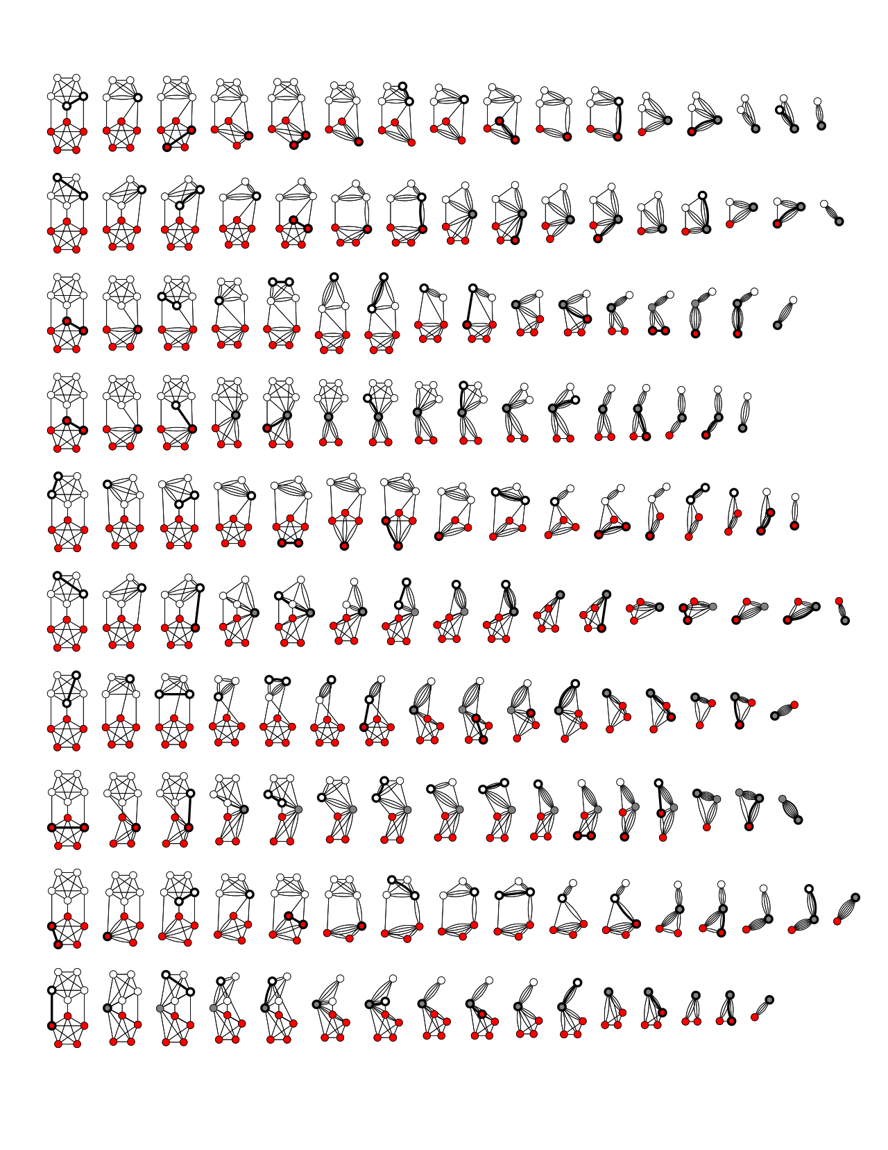
The algorithm performs the following steps

• Perform N * ln(N) contractions of the graph, where N is the total number of graph nodes
  • Record the resulting minimum-cut per contraction
  • Compare result to current min-cut and if smaller make new min-cut the current
• Return the smallest minimum-cut recorded

The below image shows 10 repetitions of the contraction procedure. The 5th repetition finds the minimum cut of size 3

Implementation approach

Given that we have a way to contract a graph down to two node subsets, all we have to do is to perform N*log(N) trials in order to find the minimum cut.

    fn minimum_cut(&self) -> Option<Graph> {

        // calculate the number of iterations as N*log(N)
        let nodes = self.nodes.len();
        let mut iterations = nodes as u32 * nodes.ilog2();
        println!("Run Iterations: {iterations}");

        // initialise min-cut min value and output as Option
        let mut min_cut = usize::MAX;
        let mut result = None;
        let repetitions = iterations as f32;

        // iterate N*log(N) time or exit if min-cut found has only 2 edges
        let mut f = f32::MAX;
        while iterations != 0 && f > 0.088 {

            // contract the graph
            if let Some(graph) = self.contract_graph() {

                // extract the number of edges
                let edges = graph.export_edges();
                // count the edges
                let edges = edges.len();

                // if number of edges returned is smaller than current
                // then store the min-cut returned from this iteration
                if edges < min_cut {
                    min_cut = edges;
                    result = Some(graph);
                    f = (min_cut as f32).div(repetitions);
                    println!("({iterations})({f:.3}) Min Cut !! => {:?}", edges);
                }
        }
            iterations -= 1;
        }
        result
    }

Graph Contraction Algorithm

Graph contraction is a technique for computing properties of graph in parallel. As its name implies, it is a contraction technique, where we solve a problem by reducing to a smaller instance of the same problem. Graph contraction is especially important because divide-and-conquer is difficult to apply to graphs efficiently. The difficulty is that divide-and-conquer would require reliably partitioning the graph into smaller graphs. Due to their irregular structure, graphs are difficult to partition. In fact, graph partitioning problems are typically NP-hard.¹

How to contract a graph

The algorithm performs the following steps

• STEP 1: Initialise temporary super node and super edge structures
• STEP 2: Contract the graph, until 2 super nodes are left
  • STEP A: select a random edge
  • STEP B : Contract the edge by merging the edge's nodes
  • STEP C : Collapse/Remove newly formed edge loops since src & dst is the new super node
  • STEP D : Identify all edges affected due to the collapsing of nodes
  • STEP E : Repoint affected edges to the new super node
• STEP 3 : find the edges between the two super node sets

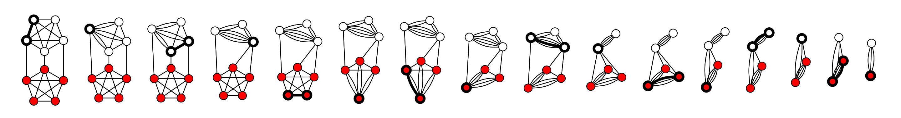
A visual example is the below image which shows the successful run of the contraction algorithm on a 10-vertex graph. The minimum cut has size 3.

Implementation approach

The key to the implementation is to

• process all nodes and their edges, so you end up with two super-sets of nodes
• finally calculate the graph edges crossing the two node super-sets

Helper Data Structures

Therefore, the following temporary data structures are necessary

• Super-nodes : HashMap holding [KEY:super-node, VALUE:set of merged nodes]
• Super-edges : list of edges in the form of HashBag that holds hash pairs of [VALUE:(source:super-node, destination:super-node)]

Worth noting here that

• We must be in a position to deal with repeating (2..*) super-edges resulting from the contraction of two super-nodes, hence the use HashBag which is an unordered multiset implementation. Use of HashSet results to elimination of super-edge multiples hence diminishing algorithm's statistical ability to produce the optimal graph contraction
• We must account for SuperEdges multiples while we (a) remove loops and (b) re-aligning super-edges following two super-node contraction

The following implementation of Super-Edges structure, provides and abstracts, the key operations of edge collapsing that is

• extract a random edge for the total set
• removal of an explicit edge
• repositioning of edges from one node onto another

#[derive(Debug)]
pub struct SuperEdges {
    list: HashMap<Node, HashBag<NodeType>>,
    length: usize
}

impl SuperEdges {

    pub fn get_random_edge(&self) -> Edge {
        let mut idx = thread_rng().gen_range(0..self.length);

        let mut iter = self.list.iter();
        if let Some((idx, &node, edges)) = loop {
            if let Some((node,edges)) = iter.next() {
                if idx < edges.len() {
                    break Some((idx, node, edges))
                }
                idx -= edges.len();
            } else {
                break None
            }
        } {
            Edge(
                node,
                edges.iter()
                    .nth(idx)
                    .copied()
                    .unwrap_or_else(|| panic!("get_random_edge(): cannot get dst node at position({idx} from src({node})"))
            )
        } else {
            panic!("get_random_edge(): Couldn't pick a random edge with index({idx}) from src")
        }
    }

    pub fn remove_edge(&mut self, src: Node, dst: Node) {
        // print!("remove_edge(): {:?} IN:{:?} -> Out:", edge, self);
        let edges = self.list.get_mut(&src).unwrap_or_else(|| panic!("remove_edge(): Node({src}) cannot be found within SuperEdges"));
        self.length -= edges.contains(&dst.into());
        while edges.remove(&dst.into()) != 0 { };
        // println!("{:?}",self);
    }
    
    pub fn move_edges(&mut self, old: Node, new: Node) {
        // Fix direction OLD -> *
        let old_edges = self.list
            .remove(&old)
            .unwrap_or_else(|| panic!("move_edges(): cannot remove old node({old})"));
        // print!("move_edges(): {old}:{:?}, {new}:{:?}", old_edges,self.list[&new]);
        self.list.get_mut(&new)
            .unwrap_or_else(|| panic!("move_edges(): failed to extend({new}) with {:?} from({new})", old_edges))
            .extend( old_edges.into_iter());

        // Fix Direction * -> OLD
        self.list.values_mut()
            .filter_map( |e| {
                let count = e.contains(&old.into());
                if  count > 0  { Some((count, e)) } else { None }
            })
            .for_each(|(mut count, edges)| {
                while edges.remove(&old.into()) != 0 {};
                while count != 0 { edges.insert(new.into()); count -= 1; }
            });
        // println!(" -> {:?}",self.list[&new]);
    }
}

Similarly, the SuperNodes structure, provides and abstracts

• the merging of two nodes into a super node
• indexed access to super nodes
• iterator

#[derive(Debug)]
/// Helper Structure that holds the `set` of merged nodes under a super node `key`
/// The HashMap therefore is used as [Key:Super Node, Value: Set of Merged Nodes]
/// A super node's set is a `Graph Component` in itself, that is, you can visit a Node from any other Node within the set
pub struct SuperNodes {
    super_nodes:HashMap<Node,HashSet<Node>>
}
impl Clone for SuperNodes {
    fn clone(&self) -> Self {
        SuperNodes { super_nodes: self.super_nodes.clone() }
    }
}
impl SuperNodes {
    /// Total size of `Graph Components`, that is, super nodes
    pub fn len(&self) -> usize { self.super_nodes.len() }
    /// Given an Graph node, the function returns the Super Node that it belongs
    /// for example given the super node [Key:1, Set:{1,2,3,4,5}]
    /// querying for node `3` will return `1` as its super node
    pub fn find_supernode(&self, node: &Node) -> Node {
        // is this a super node ?
        if self.contains_supernode(node) {
            // if yes, just return it
            *node
        } else {
            // otherwise find its super node and return it
            // get an Iterator for searching each super node
            let mut sets = self.super_nodes.iter();
            loop {
                // If next returns [Super Node, Node Set] proceed otherwise exist with None
                let Some((&src, set)) = sets.next() else { break None };
                // Is the queried Node in the set ?
                if set.contains(node) {
                    // yes, return the super node
                    break Some(src)
                }
            }.unwrap_or_else(|| panic!("find_supernode(): Unexpected error, cannot find super node for {node}"))
        }
    }
    /// Returns the graph component, aka `set` of nodes, for a given super node `key`,
    /// otherwise `None` if it doesn't exist
    pub fn contains_supernode(&self, node: &Node) -> bool {
        self.super_nodes.contains_key(node)
    }
    /// The function takes two super nodes and merges them into one
    /// The `dst` super node is merged onto the `src` super node
    pub fn merge_nodes(&mut self, src:Node, dst:Node) -> &mut HashSet<Node> {
        // remove both nodes that form the random edge and
        // hold onto the incoming/outgoing edges
        let super_src = self.super_nodes.remove(&src).unwrap();
        let super_dst = self.super_nodes.remove(&dst).unwrap();

        // combine the incoming/outgoing edges for attaching onto the new super-node
        let super_node = super_src.union(&super_dst).copied().collect::<HashSet<Node>>();
        // re-insert the src node as the new super-node and attach the resulting union
        self.super_nodes.entry(src).or_insert(super_node)
    }
    /// Provides an iterator that yields the Node Set of each super node
    pub fn iter(&self) -> SuperNodeIter {
        SuperNodeIter { iter: self.super_nodes.iter() }
    }
}
/// Ability for SuperNode struct to use indexing for search
/// e.g super_node[3] will return the HashSet corresponding to key `3`
impl Index<Node> for SuperNodes {
    type Output = HashSet<Node>;
    fn index(&self, index: Node) -> &Self::Output {
        &self.super_nodes[&index]
    }
}

/// HashNode Iterator structure
pub struct SuperNodeIter<'a> {
    iter: hash_map::Iter<'a, Node, HashSet<Node>>
}

/// HashNode Iterator implementation yields a HashSet at a time
impl<'a> Iterator for SuperNodeIter<'a> {
    type Item = &'a HashSet<Node>;

    fn next(&mut self) -> Option<Self::Item> {
        if let Some(super_node) = self.iter.next() {
            Some(super_node.1)
        } else { None }
    }
}

The SuperEdges and SuperNodes structures are initiated from the Graph structure

/// Helper Graph functions
impl Graph {
    /// SuperEdges Constructor
    pub fn get_super_edges(&self) -> SuperEdges {
        let mut length = 0;
        let list = self.edges.iter()
            .map(|(&n,e)| (n, e.iter().copied().collect::<HashBag<NodeType>>())
            )
            .inspect(|(_,c)| length += c.len() )
            .collect();
        // println!("get_super_edges(): [{length}]{:?}",list);
        SuperEdges { list, length }
    }
    /// SuperNodes Constructor
    pub fn get_super_nodes(&self) -> SuperNodes {
        SuperNodes {
            super_nodes: self.nodes.iter()
                .map(|&node| (node, HashSet::<Node>::new()))
                .map(|(node, mut map)| {
                    map.insert(node);
                    (node, map)
                })
                .collect::<HashMap<Node, HashSet<Node>>>()
        }
    }
}

Putting all together

With the supporting data structures in place we are able to write the following implementation for the contraction algorithm

    fn contract_graph(&self) -> Option<Graph> {

        if self.edges.is_empty() {
            return None;
        }

        // STEP 1: INITIALISE temporary super node and super edge structures
        let mut super_edges = self.get_super_edges();
        let mut super_nodes= self.get_super_nodes();

        // STEP 2: CONTRACT the graph, until 2 super nodes are left
        while super_nodes.len() > 2 {

            // STEP A: select a random edge
                // get a copy rather a reference so we don't upset the borrow checker
                // while we deconstruct the edge into src and dst nodes
            let Edge(src,dst) = super_edges.get_random_edge();
            // println!("While: E({src},{dst}):{:?}",super_edges.list);

            // STEP B : Contract the edge by merging the edge's nodes
                // remove both nodes that form the random edge and
                // hold onto the incoming/outgoing edges
                // combine the incoming/outgoing edges for attaching onto the new super-node
                // re-insert the src node as the new super-node and attach the resulting union
            super_nodes.merge_nodes(src, dst.into());

            // STEP C : Collapse/Remove newly formed edge loops since src & dst is the new super node
            super_edges.remove_edge( src, dst.into());
            super_edges.remove_edge( dst.into(), src);

            // STEP D : Identify all edges that still point to the dst removed as part of collapsing src and dst nodes
            // STEP E : Repoint all affected edges to the new super node src
            super_edges.move_edges(dst.into(), src);
        }

        // STEP 3 : find the edges between the two super node sets
        let mut snode_iter = super_nodes.iter();
        Some(
            self.get_crossing_edges(
                snode_iter.next().expect("There is no src super node"),
                snode_iter.next().expect("There is no dst super node")
            )
        )
    }

Finding Graph Edges between two sets of Nodes

Given subsets of nodes, in order to find the crossing edges we have to

• For each src:node in the node subset A
  • Extract the graph's edges originating from the src:node
  • Test for the intersection of graph's edges (aka destination nodes) against the node subset B
  • if the intersection is empty proceed, otherwise store the edges in a new graph

Worth noting here that for every edge found we need to account for its opposite self, for example, for Edge(2,3) we need to also add Edge(3,2)

The below function returns the edges of a graph crossing two node subsets.

    /// Given two Super Node sets the function returns the crossing edges as a new Graph structure
    fn get_crossing_edges(&self, src_set: &HashSet<Node>, dst_set: &HashSet<Node>) -> Graph {
         src_set.iter()
            .map(|src|
                ( src,
                  // get src_node's edges from the original graph
                  self.edges.get(src)
                      .unwrap_or_else(|| panic!("get_crossing_edges(): cannot extract edges for node({src}"))
                      .iter()
                      .map(|&ntype| ntype.into() )
                      .collect::<HashSet<Node>>()
                )
            )
            .map(|(src, set)|
                // Keep only the edges nodes found in the dst_set (intersection)
                // we need to clone the reference before we push them
                // into the output graph structure
                (src, set.intersection(dst_set).copied().collect::<HashSet<Node>>())
            )
            .filter(|(_, edges)| !edges.is_empty() )
            .fold(Graph::new(), |mut out, (&src, edges)| {
                // println!("Node: {node} -> {:?}",edges);
                // add edges: direction dst -> src
                edges.iter()
                    .for_each(|&dst| {
                        out.nodes.insert(dst);
                        out.edges.entry(dst)
                            .or_default()
                            .insert(src.into() );
                    });
                // add edges: direction src -> dst
                out.nodes.insert(src);
                out.edges.insert(
                    src,
                    edges.into_iter().map(|edge| edge.into()).collect()
                );
                out
            })
        // println!("Crossing graph: {:?}", output);
    }

References:

Graph Search Algorithms

The term graph search or graph traversal refers to a class of algorithms based on systematically visiting the vertices of a graph that can be used to compute various properties of graphs

To motivate graph search, let’s first consider the kinds of properties of a graph that we might be interested in computing. We might want to determine

• if one vertex is reachable from another. Recall that a vertex u is reachable from v if there is a (directed) path from v to u
• if an undirected graph is connected,
• if a directed graph is strongly connected—i.e. there is a path from every vertex to every other vertex
• the shortest path from a vertex to another vertex.

These properties all involve paths, so it makes sense to think about algorithms that follow paths. This is effectively the goal of graph-search

Processing state of graph nodes

In most case, we have to maintain some form of processing state while we perform a graph search. The most common processing data that we need to calculate and store is

• A node's visiting state
• The parent node, that is, the node we are visiting from
• A unit in terms of cost or distance

The Tracker structure holds the processed graph information while provides the means to

• access a node as an index in the form of tracker[node]
• set and update the path cost to a specific node
• set and update the parent node for the path cost calculation
• extract the minimum cost path given a target node The below code implements the above functionality

#[derive(Debug,Copy,Clone,PartialEq)]
pub enum NodeState {
    Undiscovered,
    Discovered,
    Processed
}
#[derive(Debug,Clone)]
pub struct NodeTrack {
    visited:NodeState,
    dist:Cost,
    parent:Option<Node>
}
impl NodeTrack {
    pub fn visited(&mut self, s:NodeState) -> &mut Self {
        self.visited = s; self
    }
    pub fn distance(&mut self, d:Cost) -> &mut Self {
        self.dist = d; self
    }
    pub fn parent(&mut self, n:Node) -> &mut Self {
        self.parent =Some(n); self
    }
    pub fn is_discovered(&self) -> bool {
        self.visited != NodeState::Undiscovered
    }
}
#[derive(Debug)]
pub struct Tracker {
    list: HashMap<Node, NodeTrack>
}
pub trait Tracking {
    fn extract(&self, start:Node) -> (Vec<Node>, Cost) {
        (self.extract_path(start), self.extract_cost(start))
    }
    fn extract_path(&self, start: Node) -> Vec<Node>;
    fn extract_cost(&self, start: Node) -> Cost;
}
impl Tracking for Tracker {
    fn extract_path(&self, start:Node) -> Vec<Node> {
        let mut path = VecDeque::new();
        // reconstruct the shortest path starting from the target node
        path.push_front(start);
        // set target as current node
        let mut cur_node= start;
        // backtrace all parents until you reach None, that is, the start node
        while let Some(parent) = self[cur_node].parent {
            path.push_front(parent);
            cur_node = parent;
        }
        path.into()
    }
    fn extract_cost(&self, start:Node) -> Cost {
        self[start].dist
    }
}
impl Index<Node> for Tracker {
    type Output = NodeTrack;

    fn index(&self, index: Node) -> &Self::Output {
        self.list.get(&index).unwrap_or_else(|| panic!("Error: cannot find {index} in tracker {:?}", &self))
    }
}
impl IndexMut<Node> for Tracker {
    fn index_mut(&mut self, index: Node) -> &mut Self::Output {
        self.list.get_mut(&index).unwrap_or_else(|| panic!("Error: cannot find {index} in tracker"))
    }
}

To initialise the Tracker we use the Graph structure

impl Graph {

    pub fn get_tracker(&self, visited: NodeState, dist: Cost, parent: Option<Node>) -> Tracker {
        Tracker {
            list: self.nodes.iter()
                .fold(HashMap::new(), |mut out, &node| {
                    out.entry(node)
                        .or_insert(NodeTrack { visited, dist, parent });
                    out
                })
        }
    }
}

Abstracting Breadth First Search

Breadth First Search is applied on a number of algorithms with the same pattern, that is:

1. Initiate processing state with starting node
2. Do some work on the node before exploring any paths
3. For each edge off this node
   1. Process the edge before performing search on it
   2. Push edge node on the queue for further processing
4. Do some work on the node after all edges has been discovered

Different path search algorithms have different demands in terms of

• Queue type, that is, FIFO, LIFO, etc
• Initiation states for starting node
• Pre-processing & post-processing logic required for nodes and edges

The above can be observed on how the Graph State realises the BFSearch trait for Minimum Path Cost and Shortest Distance implementation

Implementation

As a result, we can define a trait for any Graph State structure, that provides the means of how the queue processing, node & edge pre-processing / post-processing steps should be performed and in relation to the required state and behaviour.

/// Breadth First Search abstraction, that can be used to find shortest distance, lowest cost paths, etc
/// The `Path_Search()` default implementation uses the below functions while it leaves their behaviour to the trait implementer
/// - initiate step fn()
/// - Queue push & pop step fn()
/// - Queue-to-Node and vice versa step fn()
/// - Node pre/post-processing step fn()
/// - Edge pre-processing step fn()
/// - Path return fn()
/// - node state fn()
trait BFSearch {
    type Output;
    type QueueItem;

    /// Initialise the Path search given the starting node
    fn initiate(&mut self, start:Node) -> &mut Self;

    /// Pull an Item from the queue
    fn pop(&mut self) -> Option<Self::QueueItem>;

    /// Extract Node value from a Queued Item
    fn node_from_queued(&self, qt: &Self::QueueItem) -> Node;

    /// Pre-process item retrieved from the queue and before proceeding with queries the Edges
    /// return true to proceed or false to abandon node processing
    fn pre_process_node(&mut self, _node: Node) -> bool { true }

    /// Process node after all edges have been processes and pushed in the queue
    fn post_process_node(&mut self, _node: Node) { }

    /// Has the node been Discovered ?
    fn is_discovered(&self, _node: NodeType) -> bool;

    /// Process the Edge node and
    /// return 'true' to proceed with push or 'false' to skip the edge node
    fn pre_process_edge(&mut self, src: Node, dst: NodeType) -> bool;

    /// Construct a Queued Item from the Node
    fn node_to_queued(&self, node: Node) -> Self::QueueItem;

    /// Push to the queue
    fn push(&mut self, item: Self::QueueItem);

    /// Retrieve path
    fn extract_path(&self, start: Node) -> Self::Output;

    /// Path Search Implementation
    fn path_search(&mut self, g: &Graph, start: Node, goal:Node) -> Option<Self::Output> {
        // initiate BFSearch given a start node
        self.initiate(start);
        // until no items left for processing
        while let Some(qt) = self.pop() {
            //Extract the src node
            let src = self.node_from_queued(&qt);
            // pre-process and if false abandon and proceed to next item
            if !self.pre_process_node(src) { continue };
            // if we have reached our goal return the path
            if src == goal {
                return Some(self.extract_path(goal))
            }
            // given graph's edges
            // get src node's edges and per their NodeType
            if let Some(edges) = g.edges.get(&src) {
                edges.iter()
                    .for_each(|&dst| {
                        // if dst hasn't been visited AND pre-processing results to true,
                        // then push to explore further
                        if !self.is_discovered(dst)
                            && self.pre_process_edge(src, dst) {
                            // push dst node for further processing
                            self.push(self.node_to_queued(dst.into()))
                        }
                    });
                // Process node after edges have been discovered and pushed for further processing
                self.post_process_node(src);
            }
        }
        None
    }
}

Shortest Distance Path

In this case, we want to determine if one vertex is reachable from another. Recall that a vertex u is reachable from v if there is a (directed) path from v to u.¹

Search Strategy: Breadth First Search (BFS) Algorithm

The breadth-first algorithm is a particular graph-search algorithm that can be applied to solve a variety of problems such as

• finding all the vertices reachable from a given vertex,
• finding if an undirected graph is connected,
• finding (in an unweighted graph) the shortest path from a given vertex to all other vertices,
• determining if a graph is bipartite,
• bounding the diameter of an undirected graph,
• partitioning graphs,
• and as a subroutine for finding the maximum flow in a flow network (using Ford-Fulkerson’s algorithm).

As with the other graph searches, BFS can be applied to both directed and undirected graphs.

BFS Approach

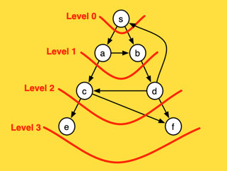
The idea of breadth first search is to start at a source vertex s and explore the graph outward in all directions level by level, first visiting all vertices that are the (out-)neighbors of s (i.e. have distance 1 from s), then vertices that have distance two from s, then distance three, etc. More precisely, suppose that we are given a graph G and a source s. We define the level of a vertex v as the shortest distance from s to v, that is the number of edges on the shortest path connecting s to v.

The above animated image provides an insight into the processing steps

• Starting node a is pushed to the queue with level set to 0
• Pop the (node,level) from the queue; at first this is (a,0)
  • Mark node as visited (black)
  • For each edge coming off the node
    • If edge is not visited
      • calculate edge-level as one edge away from node, that is, level + 1
      • push (edge, edge-level) at the end of the queue for processing (gray)

As a result and as depicted below, at the end of the graph processing, all nodes have been allocated into depth levels

Implementation

We still need to have the means to maintain the following information while we are searching the graph

• node state, in terms of processed / not processed
• parent node, that is, the node we visited from
• unit in terms of distance / level

The Tracker structure simplifies managing the node processing state of the graph, and we will use as part of our implementation.

Both Tracker and VecDeque structures are part the Graph processing State structure PDState which in turn, implements the BFSearch abstraction

As a result, the following implementation realises the BFS algorithm

    fn path_distance(&self, start:Node, goal:Node) -> Option<(Vec<Node>, Cost)> {
        /// Structure for maintaining processing state while processing the graph
        struct PDState {
            tracker: Tracker,
            queue: VecDeque<Node>
        }
        /// State Constructor from a given Graph and related the initiation requirements for the algo
        impl PDState {
            fn new(g: &Graph) -> PDState {
                PDState {
                    tracker: g.get_tracker(Undiscovered, 0, None),
                    queue: VecDeque::<Node>::new()
                }
            }
        }
        /// Implementation of Path Search abstraction
        impl BFSearch for PDState {
            type Output = (Vec<Node>, Cost);
            type QueueItem = Node;

            /// Initiate search by pushing starting node and mark it as Discovered
            fn initiate(&mut self, node:Node) -> &mut Self {
                self.queue.push_back(node);
                self.tracker[node].visited(Discovered);
                self
            }

            /// Get the first item from the start of the queue
            fn pop(&mut self) -> Option<Self::QueueItem> { self.queue.pop_front() }

            /// extract Node from the queued Item
            fn node_from_queued(&self, node: &Self::QueueItem) -> Node { *node }

            /// Has it seen before ?
            fn is_discovered(&self, node: NodeType) -> bool { self.tracker[node.into()].is_discovered() }

            /// Process Edge before pushing it at the end of the queue
            fn pre_process_edge(&mut self, src: Node, dst: NodeType) -> bool {
                let level = self.tracker[src].dist + 1;
                // mark visited, calculate distance & store parent for distance
                self.tracker[dst.into()].visited(Discovered)
                    .distance(level)
                    .parent(src);
                true
            }

            /// Construct queued item from Node
            fn node_to_queued(&self, node: Node) -> Self::QueueItem { node }

            /// Push item at the end of the queue
            fn push(&mut self, item: Self::QueueItem) { self.queue.push_back(item) }

            /// Extract path discovered so far
            fn extract_path(&self, start: Node) -> Self::Output { self.tracker.extract(start) }
        }

        // Construct the state structure and search for a path that exists between start -> goal
        PDState::new(self).path_search(self, start, goal )
    }

References:

Dijkstra's Minimum Path Cost

Here we cover problems involving finding the shortest path between vertices in a graph with weights (lengths) on the edges. One obvious application is in finding the shortest route from one address to another, however shortest paths have many other application¹

Dijkstra's Algorithm

Dijkstra’s is an important algorithm both because it is an efficient algorithm for an important problem, but also because it is a very elegant example of an efficient greedy algorithm that generates optimal solutions on a nontrivial task.

The below animated image demonstrated how the algorithm works

The above depiction performs the below steps

• push the starting node a in the priority queue with cost 0
• Pop the node with the lowest cost in the queue; at fist this is a
  • if the 'node' matches our target node b
    • extract path with minimum cost
    • terminate
  • For each edge node attached to the node
    • calculate cost distance
    • if edge node has cost larger to the calculated cost distance then assign cost to edge node, otherwise do not update cost
    • push (edge node, cost) to the priority queue and repeat

Prioritised Queue

Dijkstra's differentiating approach is that we must always process next the node with the lowest cost in the queue. To achieve this we have to make use of the BinaryHeap collection structure. The use of such structure help us to maintain on ordered-queue by node-cost, hence keeping the node with lowest-cost at the top of the heap/queue.

#[derive(Debug,Clone,Copy,Hash,Eq,PartialEq)]
pub enum NodeType {
    N(Node),
    NC(Node, Cost)
}
impl From<NodeType> for Node {
    fn from(nt: NodeType) -> Self {
        match nt { NodeType::N(node)|NC(node, _) => node }
    }
}
impl From<Node> for NodeType {
    fn from(value: Node) -> Self {
        NodeType::N(value)
    }
}
impl Ord for NodeType {
    fn cmp(&self, other: &Self) -> Ordering {
        other.partial_cmp(self).unwrap_or_else(|| panic!("Edge::cmp() - cannot compare nodes with type NodeType::N"))
    }
}
impl PartialOrd for NodeType {
    fn partial_cmp(&self, other: &Self) -> Option<Ordering> {
        match other {
            NodeType::N(_) => None,
            NC(_, cost) => {
                let NC(_,sc) = self else { panic!("Edge::partial_cmp() - cannot compare NodeType::NC against NodeType::N") };
                Some(cost.cmp(sc))
            }
        }
    }
}

Implementation

With the ordered-queue logic in place, we still need to have the means to maintain the following information per node and while we are searching the graph

• node state, in terms of processed / not processed
• parent node, that is, the node we visited from
• unit in terms of cost or distance

The Tracker structure simplifies managing the node processing state of the graph, and we will use as part of our implementation.

Both Tracker and BinaryHeap structures are part the Graph processing State structure PSState which in turn, implements the BFSearch abstraction

As a result, the algorithm can now be realised by the following implementation

    fn path_shortest(&self, start: Node, goal: Node) -> Option<(Vec<Node>, Cost)> {
        /// Structure for maintaining processing state while processing the graph
        struct PSState {
            tracker: Tracker,
            queue: BinaryHeap<NodeType>
        }

        /// State Constructor from a given Graph and related shortest path initiation requirements
        impl PSState {
            fn new(g:&Graph) -> PSState {
                PSState {
                    // reset all node costs to MAX value with no path-parent nodes
                    tracker: g.get_tracker(Undiscovered, Cost::MAX, None),
                    // We are using a BinaryHeap queue in order to always have first in the queue
                    // the node with lowest cost to explore next
                    queue: BinaryHeap::new()
                }
            }
        }

        /// Implementation of Path Search abstraction
        impl BFSearch for PSState {
            type Output = (Vec<Node>,Cost);
            type QueueItem = NodeType;

            /// Processing of starting node
            fn initiate(&mut self, start: Node) -> &mut Self {
                // set cost at start node to zero with no parent node
                self.tracker[start].distance(0);
                // push start node in the BinaryHeap queue
                self.queue.push(NC(start,0));
                self
            }

            /// get the element with the lowest cost from the queue
            fn pop(&mut self) -> Option<Self::QueueItem> { self.queue.pop() }

            /// extract node from the queued item retrieved
            fn node_from_queued(&self, qt: &Self::QueueItem) -> Node {
                (*qt).into()
            }

            /// Process current node after all edges have been discovered and marked for processing
            fn post_process_node(&mut self, node: Node) {
                self.tracker[node].visited(Discovered);
            }

            /// has the given node been seen before ?
            fn is_discovered(&self, node: NodeType) -> bool { self.tracker[node.into()].is_discovered() }

            /// Process given edge and return `true` to proceed or `false` to abandon further edge processing
            fn pre_process_edge(&mut self, src:Node, dst: NodeType) -> bool {
                if let NC(dst, cost) = dst {
                    // calc the new path cost to edge
                    let edge_cost = self.tracker[src].dist + cost;
                    // if new cost is better than previously found
                    if edge_cost > self.tracker[dst].dist  {
                        // Do no process this edge any further
                        false
                    }
                    else {
                        // set the new lower cost @node along with related parent Node
                        self.tracker[dst].distance(edge_cost).parent(src);
                        // and ensure the edge is processed further
                        true
                    }
                }
                else {
                    // somehow we got the wrong NodeType here
                    panic!("pre_process_edge(): Must use NodeType::NC")
                }
            }

            /// Construct the item to be queued, that is, (Node,Cost)
            fn node_to_queued(&self, node: Node) -> Self::QueueItem {
                NC(node, self.tracker[node].dist )
            }

            /// Push into (Node,Cost) into the queue
            fn push(&mut self, item: Self::QueueItem) { self.queue.push(item) }

            /// Get search path discovered so far
            fn extract_path(&self, start: Node) -> Self::Output { self.tracker.extract(start) }
        }

        // Construct the state structure and search for a path that exists between start -> goal
        PSState::new(self).path_search(self,start,goal)

    }

References:

Abstracting Depth First Search

Depth First Search is applied on a number of algorithms with the same pattern

1. Do some work on the node before exploring any paths
2. For edge of the node
   1. Process the edge before performing search on it
   2. Perform search on the edge
   3. Process the edge after all paths from this edge, got explored
3. Do some work on the node after all paths from this node, got explored

Different algorithms have different demands on how what the graph state should be and which of those steps are required and in what way

The above can be observed on how the Graph State realises the DFSearch trait for Topological sort and Strongly Connected Components implementation

Implementation

As a result, we can define a trait for any Graph State structure, that provide the means of how the pre-processing / post-processing steps should be performed and in relation to the required state and behaviour.

It is important to note here the recursive nature of the search and hence the need for self to maintain the internal state while recursively searching the graph

/// Depth First Search abstraction, enabling a variety of implementations such as, strongly connected components, topological sort, etc
/// The `Path_Search()` default implementation uses the below functions while it leaves their behaviour to the trait implementer
/// - Node pre-processing step fn()
/// - Node post-processing step fn()
/// - Node pre-processing edge fn()
/// - abort recursion fn()
/// - Path return fn()
/// - node state fn()
trait DFSearch {
    type Output;

    /// work to be done before edges are explored, that is, discovered but not processed
    /// uses incl. measuring entry time, set node state, etc
    fn pre_process_node(&mut self, node: Node) -> &mut Self;

    /// work to be done after the edges have been explored; hence the node is now processed
    /// uses incl. measuring exit time, set node parent, save node in path, etc
    fn post_process_node(&mut self, node: Node) -> &mut Self;

    /// work to be done after the node pre-processed and before the edges is explored
    /// uses incl. check for loops, categorize edge into types, etc
    /// default implementation does nothing otherwise you have to override
    fn pre_process_edge(&mut self, _edge: Edge) -> &mut Self { self }

    /// Abort the recursion
    /// uses incl. detecting the graph is not Direct acyclic, etc
    fn abort(&self) -> bool { false }

    /// return the path at position and given the pre/post processing steps
    fn path(&self) -> &Self::Output;

    /// return whether the node has been seen before
    fn is_discovered(&self, node: Node) -> bool;

    /// Default implementation of depth first search
    fn path_search(&mut self, g: &Graph, start: Node) -> Option<&Self::Output> {
        // Entering the node at time tick()
        if self.pre_process_node(start).abort() { return None }

        // processing the edges
        // println!("Enter: {start}:{:?}", self.tracker[start]);
        if let Some(edges) = g.edges.get(&start) {
            for &dst in edges {
                let d = dst;

                if self.pre_process_edge(Edge(start,d)).abort() { return None };

                if !self.is_discovered(d.into()) {
                    self.path_search(g, d.into());
                }
            }
        }
        // Exiting the node at time tick()
        if self.post_process_node(start).abort() { return None };
        // println!("Exit: {start}:{:?}", self.tracker[start]);
        Some(self.path())
    }
}

Topological Sort Algorithm

A topological sort is an ordering of the nodes of a directed graph such that if there is a path from node a to node b, then node a appears before node b in the ordering.

Graph Recursion and Processing state

The idea is to go through the nodes of the graph and always begin a depth-first search at the current node if it has not been processed yet. During the searches, the nodes have three possible states:

• state 0: the node has not been processed (white)
• state 1: the node is under processing (light gray)
• state 2: the node has been processed (dark gray)

Initially, the state of each node is 0. When a search reaches a node for the first time, its state becomes 1. This is our pre-processing step for the node

If the graph contains a cycle, we will find this out during the search, because sooner or later we will arrive at a node whose state is 1. In this case, it is not possible to construct a topological sort. This is the pre-processing step for the edge.

If the graph does not contain a cycle, we can construct a topological sort by adding each node to a list when the state of the node becomes 2. This is our post-processing step for the node. This list in reverse order is a topological sort

As a result we can implement the DFSearch trait in the following way in relation to the above pre-processing & post-processing steps

/// Graph state that we need to maintain
/// for the topological sort algorithm
struct TState {
    tracker: Tracker,
    path: Vec<Node>,
    abort: bool
}

impl TState {
    /// Construct a new `GraphState` given a `Graph`
    fn new(g: &Graph) -> TState {
        TState {
            tracker: g.get_tracker(Undiscovered, 0, None),
            path: Vec::new(),
            abort: false
        }
    }
}

/// Topological sort implementation of the TState
/// There is no need for exit/entry time or tracking parent node.
/// Here we only need to save the `node` in the `tracker.path` following its full processing
impl DFSearch for TState {
    type Output = Vec<Node>;

    /// mark node as visited but not processed
    fn pre_process_node(&mut self, node: Node) -> &mut Self {
        self.tracker[node].visited(Discovered);
        self
    }

    /// Important we store the node in the path following node processing complete
    fn post_process_node(&mut self, node: Node) -> &mut Self {
        self.tracker[node].visited(Processed);
        self.path.push(node);
        self
    }

    /// before we jump into the edge for further exploration
    /// we check if the edge is actually a node already `Discovered` but not `Processed`
    /// if that is the case, we set the abort flag to `True`
    fn pre_process_edge(&mut self, edge: Edge) -> &mut Self {
        let Edge(_,dst) = edge;
        if self.tracker[dst.into()].visited == Discovered {
            self.abort = true;
        }
        self
    }

    /// Implement the abort fn() so we can stop the path search recursion
    fn abort(&self) -> bool {
        self.abort
    }

    /// extract the aggregate path stored
    fn path(&self) -> &Self::Output {
        &self.path
    }

    /// return true if node is either `Discovered` or `Processed`
    fn is_discovered(&self, node: Node) -> bool {
        self.tracker[node].is_discovered()
    }
}

Implementation

When the search has completed and has exhausted all paths the path member of the Tracker structure will now contain the order by which the nodes have been visited. As a result we only have to reverse such order and return it.

/// Topological Sort trait
pub trait TopologicalSort {
    fn topological_sort(&self) -> Option<Vec<Node>>;
}
/// Graph implementation of Topological Sort
impl TopologicalSort for Graph {
    /// Implementation of topological sort for Graph
    fn topological_sort(&self) -> Option<Vec<Node>> {
        // initiate the run state structure for calculating the topological sort of the graph
        let mut ts = TState::new(self);

        // Construct a path aggregate, that is, each path found is joined up together
        // achieved by appending the path of each iteration onto tracker.path
        // see post_processing() of TState implementation of DFSearch
        for &node in &self.nodes {
            // if node is not yet visited && search hasn't thrown a NONE, that is, we've found a circle
            if !ts.is_discovered(node)
                && ts.path_search(self, node).is_none() {
                return None
            }
        }

        // Extract & reverse path from tracker so we extract the topological sort
        ts.path.reverse();
        Some(ts.path)
    }
}

Strong Connectivity

In a directed graph, the edges can be traversed in one direction only, so even if the graph is connected, this does not guarantee that there would be a path from a node to another node. For this reason, it is meaningful to define a new concept that requires more than connectivity.

A graph is strongly connected if there is a path from any node to all other nodes in the graph. The strongly connected components of a graph divide the graph into strongly connected parts that are as large as possible. The strongly connected components form an acyclic component graph that represents the deep structure of the original graph.

The yellow directed acyclic graph is the condensation of the blue directed graph. It is formed by contracting each strongly connected component of the blue graph into a single yellow vertex

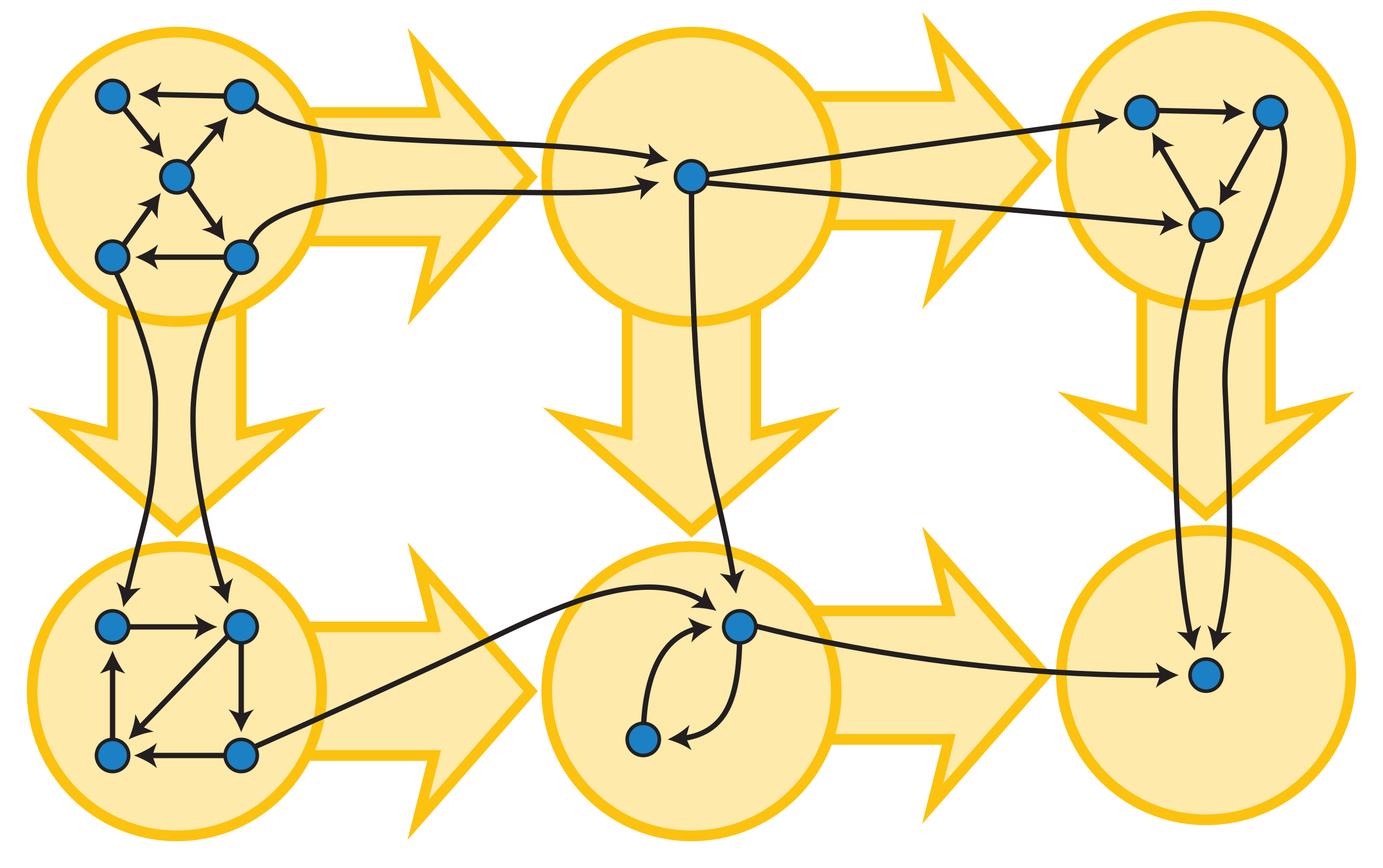
Kosaraju’s algorithm

Kosaraju’s algorithm is an efficient method for finding the strongly connected components of a directed graph.

Approach

The algorithm performs two depth-first searches

1. the first search constructs an ordered node list of nodes according to the structure of the graph.
2. the second search applies the ordered node list against the reversed edges of the graph in order to find the strongly connected components.

Graph Recursion and Processing State

In the first Depth First Search we need to calculate per node

• the exit time, that is, the time in which the node has been Processed, that is, there is nothing left to be found.
• the node state in relation to any of the states, Undiscovered, Discovered or Processed

Recursion is a key implementation approach that will enable us to perform

1. Node pre-processing, e.g. capture/log the entry time and before search any deeper
2. Node post-processing, e.g. capture/log the exit time after there is no path remaining to be found from this node

As a result to measure time across recursions and without the use of a global variable, we resort to the GraphState struct that

• implements the DFSearch trait that provides the recursive function
• holds the recursion state for time, path at node, node state & ordered list

In addition, GraphState provide us with the Tracker structure that simplifies handling of the node processing state while we are search the graph.

/// GraphState struct enable us to maintain the processing state of the graph
/// and while we apply a recursive approach in searching the graph
struct GraphState {
    tracker: Tracker,
    queue: BinaryHeap<NodeType>,
    time: Cost,
    path: Vec<Node>
}

impl GraphState {
    /// Construct a new `GraphState` given a `Graph`
    fn new(g: &Graph) -> GraphState {
        GraphState {
            tracker: g.get_tracker(Undiscovered, 0, None),
            queue: BinaryHeap::new(),
            time: 0,
            path: Vec::new()
        }
    }

    /// Extract from `BinaryHeap` the exit times per ordered from max -> min
    fn get_timings(&self) -> Vec<(Node, Cost)> {
        self.queue.iter().rev().map(|&s| {
            let NC(n, c) = s else { panic!("get_timings(): node type is not NodeType::NC") };
            (n,c)
        }  ).collect::<Vec<_>>()
    }
}

/// Graph State implements DFSearch trait and particularly provides specific implementation for
/// the calculation of the strongly connected components, in terms of node post/pre processing fn(),
/// path return fn() and node state fn()
impl DFSearch for GraphState {
    type Output = Vec<Node>;

    /// capture time of entry and set node state to visited,
    /// given the node's edges have yet be visited
    fn pre_process_node(&mut self, node: Node) -> &mut Self {
        // Entering the node at time tick()
        self.time += 1;
        self.tracker[node].visited(Discovered).distance(self.time);
        self
    }

    /// capture time of exit and set node state to processed,
    /// given all edges have also been processed
    fn post_process_node(&mut self, node: Node) -> &mut Self {
        // Exiting the node at time tick()
        self.time += 1;
        self.tracker[node].visited(Processed).distance(self.time);
        self.queue.push(NC(node, self.time));
        self.path.push(node);
        self
    }

    /// Return the path as it was calculated by the post processing step
    fn path(&self) -> &Self::Output {
        &self.path
    }

    /// return the state of the node
    fn is_discovered(&self, node: Node) -> bool {
        self.tracker[node].is_discovered()
    }
}

Transpose the graph

The GraphState will help us capture the node order by which we will run search on the second pass. However, the second pass must run against the transposed graph, that is, the graph with all edges reversed.

impl Graph {
    pub fn transpose(&self) -> Graph {
        self.nodes.iter()
            .fold(Graph::new(), |mut g, &node| {
                g.nodes.insert(node);
                // reverse the edges for this node, if any
                if let Some(edges) = self.edges.get(&node) {
                    edges.iter()
                        .for_each(|&e|{
                            g.nodes.insert(e.into());
                            g.edges.entry(e.into()).or_default().insert(node.into());
                        });
                }
                g
            })
    }
}

Final implementation

With all of the above elements in place, The below function provides an implementation approach to the algorithm

pub trait ConnectedComponents {
    fn strongly_connected(&self) -> Vec<Vec<Node>>;
}

impl ConnectedComponents for Graph {
    fn strongly_connected(&self) -> Vec<Vec<Node>> {

        // initiate the run state structure for calculating the scc of the graph
        // and in order to enable recursive searching in rust
        let mut gs = GraphState::new(self);

        // Pass 1: Find all paths and calculate entry and exit times per node
        self.nodes.iter()
            .for_each(|&start| {
                // println!("Start >> {start}");
                if !gs.tracker[start].is_discovered() {
                    let path = gs.path_search(self, start);
                    println!("Pass 1: Path {:?}",path);
                    gs.path.clear();
                }
            });

        // Extract node sequence ordered by highest exit times
        let v = gs.get_timings();
        println!("Timings: {:?}",v);
        // reverse the graph edges
        let tg = self.transpose();
        // reset run state
        gs = GraphState::new( &tg);

        // Pass 2: Identify and store each strongly connected component identified
        v.into_iter()
            .fold(Vec::new(),|mut components, (node, _)| {
                if !gs.is_discovered(node) {
                    // extract new component
                    let component = gs.path_search(&tg, node ).unwrap();
                    println!("Pass 2: Component [{}]{:?}", component.len(), component);
                    // store component found
                    components.push(component.clone() );
                    // reset path so to remove last found component
                    gs.path.clear();
                }
                components
            })
    }
}

Minimum Spanning Tree

A minimum spanning tree (MST) or minimum weight spanning tree is a subset of the edges of a connected, edge-weighted undirected graph that connects all the vertices together, without any cycles and with the minimum possible total edge weight.¹

That is, it is a spanning tree whose sum of edge weights is as small as possible.

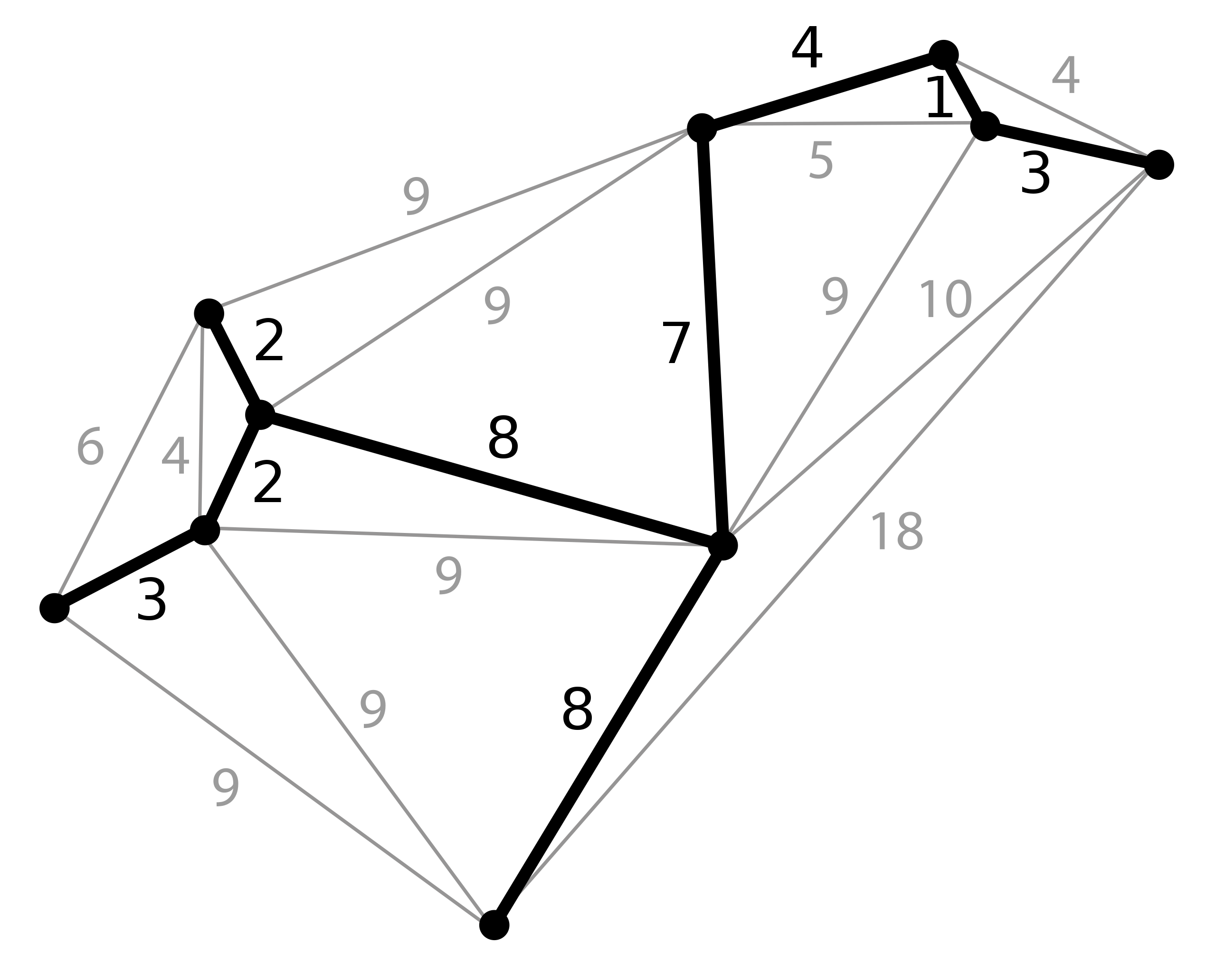More generally, any edge-weighted undirected graph (not necessarily connected) has a minimum spanning forest, which is a union of the minimum spanning trees for its connected components.

There are many use cases for minimum spanning trees. One example is a telecommunications company trying to lay cable in a new neighborhood. If it is constrained to bury the cable only along certain paths (e.g. roads), then there would be a graph containing the points (e.g. houses) connected by those paths. Some paths might be more expensive, because they are longer, or require the cable to be buried deeper; these paths would be represented by edges with larger weights

Kruskal's MST Algorithm

In Kruskal’s algorithm, we start with the spanning tree containing only the nodes of the graph and with no any edges connecting the nodes.

Then the algorithm goes through, adding the edges one at a time, ordered by their weights, and as long as the edge is not creating a cycle.

Approach

Let's look at the following input graph as an example.

The algorithm maintains the components of the tree. Initially, each node of the graph belongs to a separate component. As shown below there are six components since none of the nodes are connected.

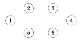
We always start with the lowest weighted edge by adding it to the tree, in this case (5,6). As result, two components are now merged into one as in the below example where nodes 5 and 6 form a new component

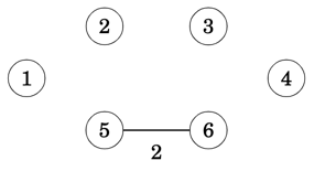
Next in order are edges (6,3),(1,2),... and so on, until finally we have added all edges in the graph, one by one and with all nodes now merged into a single component, hence the minimum spanning tree has been found

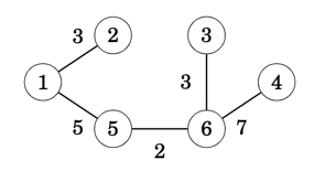
Overall the approach can be summarised as following

1. Phase 1: Sort Edges by minimum cost first
2. Phase 2: Build Minimum Spanning Tree
   1. Create an empty graph G
   2. Initiate the graph components, that is, one per node
   3. While there are > 1 graph components remaining
      1. Retrieve edge with the lowest weight (src,dst)
      2. Find component for src, let's say it is src'
      3. Find component for dst, let's say it is dst'
      4. if src' is different to dst' then
         1. Merge dst' into the src' component
         2. Add edge (src,dst) into the graph G

Super Nodes as Components

The SuperNodes struct used to solve the minimum cut algorithm is more or less the right tool in this instance given that the definition of a super node is synonymous to a graph component.

The SuperNodes structure, provides us with the

• merging of two super node components into a super node
  • finding of the super node component that a given node belongs to

#[derive(Debug)]
/// Helper Structure that holds the `set` of merged nodes under a super node `key`
/// The HashMap therefore is used as [Key:Super Node, Value: Set of Merged Nodes]
/// A super node's set is a `Graph Component` in itself, that is, you can visit a Node from any other Node within the set
pub struct SuperNodes {
    super_nodes:HashMap<Node,HashSet<Node>>
}
impl Clone for SuperNodes {
    fn clone(&self) -> Self {
        SuperNodes { super_nodes: self.super_nodes.clone() }
    }
}
impl SuperNodes {
    /// Total size of `Graph Components`, that is, super nodes
    pub fn len(&self) -> usize { self.super_nodes.len() }
    /// Given an Graph node, the function returns the Super Node that it belongs
    /// for example given the super node [Key:1, Set:{1,2,3,4,5}]
    /// querying for node `3` will return `1` as its super node
    pub fn find_supernode(&self, node: &Node) -> Node {
        // is this a super node ?
        if self.contains_supernode(node) {
            // if yes, just return it
            *node
        } else {
            // otherwise find its super node and return it
            // get an Iterator for searching each super node
            let mut sets = self.super_nodes.iter();
            loop {
                // If next returns [Super Node, Node Set] proceed otherwise exist with None
                let Some((&src, set)) = sets.next() else { break None };
                // Is the queried Node in the set ?
                if set.contains(node) {
                    // yes, return the super node
                    break Some(src)
                }
            }.unwrap_or_else(|| panic!("find_supernode(): Unexpected error, cannot find super node for {node}"))
        }
    }
    /// Returns the graph component, aka `set` of nodes, for a given super node `key`,
    /// otherwise `None` if it doesn't exist
    pub fn contains_supernode(&self, node: &Node) -> bool {
        self.super_nodes.contains_key(node)
    }
    /// The function takes two super nodes and merges them into one
    /// The `dst` super node is merged onto the `src` super node
    pub fn merge_nodes(&mut self, src:Node, dst:Node) -> &mut HashSet<Node> {
        // remove both nodes that form the random edge and
        // hold onto the incoming/outgoing edges
        let super_src = self.super_nodes.remove(&src).unwrap();
        let super_dst = self.super_nodes.remove(&dst).unwrap();

        // combine the incoming/outgoing edges for attaching onto the new super-node
        let super_node = super_src.union(&super_dst).copied().collect::<HashSet<Node>>();
        // re-insert the src node as the new super-node and attach the resulting union
        self.super_nodes.entry(src).or_insert(super_node)
    }
    /// Provides an iterator that yields the Node Set of each super node
    pub fn iter(&self) -> SuperNodeIter {
        SuperNodeIter { iter: self.super_nodes.iter() }
    }
}
/// Ability for SuperNode struct to use indexing for search
/// e.g super_node[3] will return the HashSet corresponding to key `3`
impl Index<Node> for SuperNodes {
    type Output = HashSet<Node>;
    fn index(&self, index: Node) -> &Self::Output {
        &self.super_nodes[&index]
    }
}

/// HashNode Iterator structure
pub struct SuperNodeIter<'a> {
    iter: hash_map::Iter<'a, Node, HashSet<Node>>
}

/// HashNode Iterator implementation yields a HashSet at a time
impl<'a> Iterator for SuperNodeIter<'a> {
    type Item = &'a HashSet<Node>;

    fn next(&mut self) -> Option<Self::Item> {
        if let Some(super_node) = self.iter.next() {
            Some(super_node.1)
        } else { None }
    }
}

BinaryHeap for edge Ordering

To provide an ordered edge list we use the BinaryHeap collection that uses the edge's weight as the prioritisation key. The following Step implementation provide us with the desirable result.

/// BinaryHeap Step structure containing `Edge(src,(dst,cost))` tuple
/// The `cost` is only used as the prioritisation key for the `Heap`
/// Implementing MinHeap through reverse comparison of Other against Self
impl PartialOrd for Edge {
    fn partial_cmp(&self, other: &Self) -> Option<Ordering> {
        match other.1 {
            N(_) => other.partial_cmp(self),
            NC(_, cost) => {
                let Edge(_,NC(_,sc)) = self else { panic!("") };
                cost.partial_cmp(sc)
            }
        }
    }
}
impl Ord for Edge {
    fn cmp(&self, other: &Self) -> Ordering {
        self.partial_cmp(other).unwrap()
    }
}

Additionally, we have the following helper Graph functions that provide us with

• the ordered edge list
• the sum of weights for all edges in the graph
• adding an edge into the graph

    /// Sums up the cost of all weighted edges
    pub fn sum_edges(&self) -> Cost {
        self.edges
            .values()
            .fold(0, |cost, edges| {
                cost + edges.iter()
                    .map(|&dst| {
                        let NC(_,c) = dst else { panic!("get_mst_cost(): Edge destination node is not of type NodeType::NC") };
                        c
                    })
                    .reduce(|acc,c| acc + c )
                    .unwrap()
            }) >> 1 // in an undirected graph we count twice the edge hence dividing by 2
    }
    /// Adds a new Edge to the graph
    pub fn push_edge(&mut self, edge: Edge) {
        let Edge(src, dst) = edge;
        self.nodes.insert(src);
        self.edges.entry(src)
            .or_default()
            .insert(dst);
        let NC(dst,cost) = dst else { panic!("") };
        self.nodes.insert(dst);
        self.edges.entry(dst)
            .or_default()
            .insert(NC(src,cost));
    }
    /// Returns Graph's edges in the form of a MinHeap, that is,
    /// the lowest cost edge at the top of the heap
    pub fn get_edges_by_cost(&self) -> BinaryHeap<Edge> {
        self.edges.iter()
            .fold(BinaryHeap::new(), |mut heap, (&src, edges)| {
                    heap.extend(
                        edges.iter().map(|&dst| Edge(src,dst))
                    );
                    heap
                })

    }

Implementation

As a result, the following implementation consolidates all of the above into the Kruskal's algorithm implementation.

    /// MST using Kruskal's algorithm implementation
    pub fn mst_kruska(&self) -> Option<Graph> {

        // Get the ordered heap by lowest cost Edge on top
        let mut heap = self.get_edges_by_cost();
        // Keeps the graph's components, that is, a super node is a graph component's lead node
        // The initial state is for each node to be a lead component node with a component of its own
        let mut snodes = self.get_super_nodes();
        // the output graph that will hold *only* the edges
        // that form the minimum spanning tree
        let mut graph = Graph::new();

        // As long as more than 2 components
        while snodes.len() > 1 {
            // get the edge with the lowest cost
            // otherwise if we've run out of edges while there are 2 or more components
            // then the graph IS NOT CONNECTED
            let Some(edge) = heap.pop() else { return None };
            let Edge(src, NC(dst, _)) = edge else { panic!("mst_kruska() - Cannot find NodeType::NC") };
            // print!("({src:2}->{dst:2}):{cost:6} - ");

            // if src is not a super node then get its super node
            let src = snodes.find_supernode(&src);
            // if dst is not a super node then get its super node
            let dst = snodes.find_supernode(&dst);

            // if src component differs from dst component then merge the two and save the edge connecting them
            if src != dst {
                snodes.merge_nodes(src, dst);
                graph.push_edge(edge);
                // println!("Store");
            } else {
                // println!("Skip");
            }
        }
        Some(graph)
    }

Prim's MST Algorithm

Prim’s algorithm resembles Dijkstra’s algorithm. The difference is that Dijkstra’s algorithm always selects an edge whose distance from the starting node is minimum, but Prim’s algorithm simply selects the minimum weight edge that adds a new node to the tree

Approach

The algorithm first adds an arbitrary node to the tree. After this, the algorithm always chooses a minimum-weight edge that adds a new node to the tree. Finally, all nodes have been added to the tree and a minimum spanning tree has been found

To illustrate how the algorithm works let's consider the following input graph

When we start, the minimum spanning tree has no edges

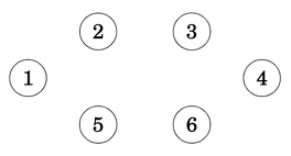
We then select an arbitrary node, in this case 1, and from edges (1,2),(1,5) we choose the edge (1,2) that has the lowest weight, and we then add it into the output tree. At this point in time, nodes [1,2] are spawned into the evolving tree.

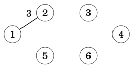
With edge (1,2) added to the tree, we're looking to all edges that cross between the tree and the non-tree nodes. In this case we have edges [(1,5),(2,5),(2,3)] with (2,3) being the one that has the lowest weight from all known crossing edges.

At this point the tree contains nodes [1,2,3] with nodes remaining outside the tree as [5,6,4]

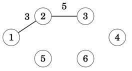
We repeat the process, always expanding one node at a time and adding to the tree the lowest weight edge each time and until there are no more nodes remaining outside the tree.

Min-Ordered edge BinaryHeap

To provide a minimum-ordered edge list, we make use of the BinaryHeap collection with the edge's weight as the prioritisation key. The following Step implementation provide us with the desirable result

/// BinaryHeap Step structure containing `Edge(src,(dst,cost))` tuple
/// The `cost` is only used as the prioritisation key for the `Heap`
/// Implementing MinHeap through reverse comparison of Other against Self
impl PartialOrd for Edge {
    fn partial_cmp(&self, other: &Self) -> Option<Ordering> {
        match other.1 {
            N(_) => other.partial_cmp(self),
            NC(_, cost) => {
                let Edge(_,NC(_,sc)) = self else { panic!("") };
                cost.partial_cmp(sc)
            }
        }
    }
}
impl Ord for Edge {
    fn cmp(&self, other: &Self) -> Ordering {
        self.partial_cmp(other).unwrap()
    }
}

Implementation

Few key points related to the below implementation

1. We hold the evolving tree in a Graph structure with its nodes HashSet representing the tree's Component for queries
2. When we spawn a new node, we don't search for the minimum weight edge, rather we store all crossing edges in the heap;
3. Edges added in the heap might go stale, that is, future iterations cause edges nodes to be pulled inside the tree component, hence when extracting the min-weight edge from the heap we need to ensure the edge isn't stale.

As a result, the following implementation consolidates all of the above into the Prim's algorithm implementation.

    /// MST using Prim's algorithm implementation
    pub fn mst_prim(&self) -> Option<Graph> {

        // Create an empty Graph/Tree to add one edge at a time
        // we'll be using g.node as the Tree's Component invariant,
        // that is, the Component that contains all vertices absorbed by the Tree
        let mut tree = Graph::new();

        // Min-Ordered heap with all edges found crossing the evolving tree
        let mut heap = BinaryHeap::<Edge>::new();

        // seed with first vertex
        let &start = self.nodes.iter().next().unwrap();
        heap.push(Edge(start, NC(start, 0)));

        // spawn a node at a time until we have spawned all graph nodes
        // while tree component isn't equal input component
        while tree.nodes != self.nodes {
            // spawn a new edge node from the queue with the smallest edge weight
            let src = match heap.pop() {
                // if the queue is empty, but still have nodes to spawn
                // then either (a) the graph is not connected or (b) is a directed graph
                None => return None,
                // spawn the destination node from edge
                Some(Edge(_, NC(dst, _))) => dst,
                Some(Edge(_, N(_))) => panic!("mst_prim(): Extracted edge using wrong NodeType::N"),
            };

            // Add all edges that are crossing the tree Component given the spawned node
            // and have not yet been spawned, that is, they are NOT already part of tree component
            heap.extend(self.edges.get(&src)
                .unwrap_or_else(|| panic!("mst_prim(): Node ({src}) has not edges; Graph is not undirected or connected"))
                .iter()
                // remove any edge node already in the mst, part of Component X
                .filter(|&&dst| !tree.nodes.contains(&dst.into()))
                // push edges crossing Component X, that is,
                // src IN Component X, dst NOT IN Component X
                .map(|&dst| Edge(src, dst))
            );

            // find the min-weigh edge that is crossing the current tree component
            // don't remove from heap as we need to spawn dst node for the next iteration
            while let Some(&edge) = heap.peek() {
                let Edge(src, dst) = edge;
                // Is this edge a stale or a valid one, that is, crosses the tree component
                if HashSet::from([src, dst.into()]).is_subset(&tree.nodes) {
                    // Some times heap holds older edges that, after few iterations they get stale,
                    // that is, both edges nodes have been moved into the tree component
                    heap.pop();
                } else {
                    // either src or dst edge nodes are outside the tree component
                    // hence add the edge into the tree
                    tree.push_edge(edge);
                    // exit the while loop since we've found the edge with the min weight
                    break
                }
            }
        }
        Some(tree)
    }

Single-linkage clustering

Single-linkage clustering is one of several methods of hierarchical clustering. It is based on grouping clusters in bottom-up fashion (agglomerative clustering), at each step combining two clusters that contain the closest pair of elements not yet belonging to the same cluster as each other. A drawback of this method is that it tends to produce long thin clusters in which nearby elements of the same cluster have small distances, but elements at opposite ends of a cluster may be much farther from each other than two elements of other clusters. This may lead to difficulties in defining classes that could usefully subdivide the data¹

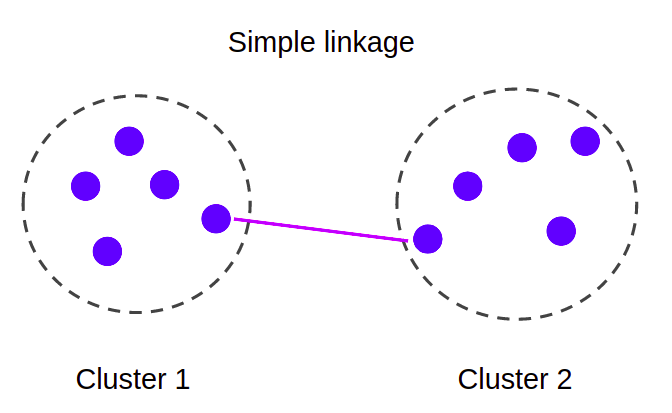
Approach

At the start all points form their own component. Then at each iteration, we fuse together those components that are connected by the shortest distance edge. We repeat until the number of components left is equal to the number of clusters required.

This is exactly how the Kruska's algorithm works, with the only difference, the produced Minimum Spanning Tree can be seen as a single component / cluster, therefore we have to stop the process until k components/clusters are left.

However, if we stop the at k components our min spanning tree won't have the remaining edges connecting the clusters, hence we won't know the clusters' spacing, that is, the distance between the closest together pair of separated nodes.

ClusterSet Structure

Therefore, we need to capture both (a) the min spanning tree and (b) the nodes forming the k clusters requested

The ClusterSet structure captures such information and further provides the means to query the spacing of a clustering, through the use of the following functions,

• crossing_edges() returns those mst edges crossing the node clusters
• spacing() returns the smallest mst edge

struct ClusterSet {
    mst: Graph,
    clusters : SuperNodes
}

impl ClusterSet {
    /// spacing of a clustering. It's the distance between the closest together pair of separated points
    /// We want all of the separated points to be as far apart as possible.
    /// That is, we want the spacing to be big. The bigger the better
    fn spacing(&self) -> Edge {
        self.crossing_edges().pop().unwrap_or_else(|| panic!("spacing(): no edges found spanning the clusters"))
    }
    fn crossing_edges(&self) -> BinaryHeap<Edge>{

        let mut input = self.mst.get_edges_by_cost();
        let mut output = BinaryHeap::<Edge>::new();

        while let Some(edge) = input.pop() {
            let Edge(src, dst) = edge;
            if self.clusters.find_supernode(&src) != self.clusters.find_supernode(&dst.into()) {
                output.push(edge);
            }
        }
        output
    }
}

Implementation

With the ClusterSet data structure in place we implemented the Graph implementation of the Clustering trait looks as follows

trait Clustering {
    fn find_clusters(&self, k: usize) -> Option<ClusterSet>;
}

impl Clustering for Graph {

    fn find_clusters(&self, k: usize) -> Option<ClusterSet> {

        // Get the ordered heap by lowest cost Edge on top
        let mut heap = self.get_edges_by_cost();
        // Keeps the graph's components, that is, a super node is a graph component's lead node
        // The initial state is for each node to be a lead component node with a component of its own
        let mut snodes = self.get_super_nodes();
        // the output graph that will hold *only* the edges
        // that form the minimum spanning tree
        let mut graph = Graph::new();
        let mut clusters = None;

        // As long as more than 2 components
        while snodes.len() > 1 {
            // get the edge with the lowest cost
            // otherwise if we've run out of edges while there are 2 or more components
            // then the graph IS NOT CONNECTED
            let Some(edge) = heap.pop() else { return None };
            let Edge(src, NC(dst, _)) = edge else { panic!("find_clusters() - Cannot find NodeType::NC") };
            // print!("({src:2}->{dst:2}):{cost:6} - ");

            // if src is not a super node then get its super node
            let src = snodes.find_supernode(&src);
            // if dst is not a super node then get its super node
            let dst = snodes.find_supernode(&dst);

            // if src component differs from dst component then merge the two and save the edge connecting them
            if src != dst {
                snodes.merge_nodes(src, dst);
                graph.push_edge(edge);
                // println!("Store");
            } else {
                // println!("Skip");
            }
            if snodes.len() == k {
                clusters = Some(snodes.clone())
            }
        }
        Some(ClusterSet{
            mst: graph,
            clusters: clusters.unwrap()
        })
    }
}